7. Peak Deconvolution

Peak deconvolution is a data analysis technique to resolve overlapping peaks in spectral data. In Raman spectroscopy, the observed spectrum often contains multiple peaks due the presence of multiple vibrations or chemical components, which, in complex samples, can overlap, hindering accurate quantification and identification of molecular entities. Applying curve-fitting to separate the overlapping peaks reveals the individual spectral and their respective contributions. In addition, peak fitting allows the precise determination of peak position and width, even in spectra with overlapping peaks, which is crucial for spectral analysis of Brillouin scattering spectra but has applications in Raman spectroscopy as well, for example when performing melting or tensile experiments or samples where the external perturbation is expected to affect peak position or shape.

This section provides an overview of the peak deconvolution techniques available in SMDExplorer, beginning with a discussion of the available line shapes and an introduction of the fitting algorithm and its parameters. After this theoretical preface, The Fitting Window describes the peak deconvolution user interface in SMDExplorer while Peak Deconvolution - A How-to provides instructions and hints how to perform a peak deconvolution analysis on a real-world dataset. This section closes with an overview of the visualization options available in SMDExplorer for display and analysis of peak deconvolution results.

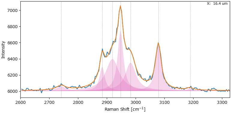
Fig. 7.1 Peak Deconvolution

7.1. Line Shapes

SMDExplorer offers the following line shapes:

• Gaussian

• Lorentzian

• Pseudo-Voigt

• Damped Harmonic Oscillator (DHO)

Peak Deconvolution - Line Shapes illustrates the different shape of the first three line shapes.

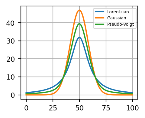
Fig. 7.2 Peak Deconvolution - Line Shapes

Each peak is characterized by three parameters:

• peak amplitude. This describes area under the curve of the peak.

• peak position. This describes the location of the highest value of the peak.

• peak width. The characteristic width of the peak.

The meaning of the three parameters is illustrated in Anatomy of a Peak, where \(\mu\) represents peak position, \(A\) peak amplitude, and \(\sigma\) peak width.

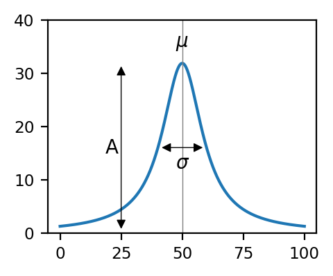
Fig. 7.3 Anatomy of a Peak

To make comparison between the different line shapes easier, the full width at half maximum (FWHM) is commonly used.

7.1.1. Gaussian

(7.1)\[ f(x) = \frac{A}{\sigma \sqrt{2 \pi}} e^{-(x-\mu)^2 /\ 2 \sigma^2} \]

Here (7.1), \(A\) is the Gaussian’s amplitude, \(\mu\) the peak position, and \(\sigma\) the peak width with a full width at half maximum (FWHM) of \(2 \sigma \sqrt{2\cdot \ln2}\).

7.1.2. Lorentzian

(7.2)\[ f(x) = \frac{A}{\pi} \frac{\sigma}{(x-\mu)^2+\sigma^2} \]

Here (7.2), \(A\) is the Lorentzian’s amplitude, \(\mu\) the peak position, and \(\sigma\) the peak width with a FWHM of \(2 \sigma\).

See also

The Lorentzian (GPU) lineshape is mathematically identical to the conventional Lorentzian curve. Parameter optimization is, however, performed on the computer’s GPU rather than the CPU, which allows highly-parallel processing and can lead to significant performance gains.

7.1.3. Pseudo-Voigt

The Pseudo-Voigt line shape is a weighted sum of a Gaussian and Lorentzian distribution with common amplitude, peak position, and FWHM. This line shape is commonly used to describe the convolution of a Lorentzian scattering peak with a Gaussian instrument function.

(7.3)\[ f(x) = \frac{(1-\alpha)\cdot A}{\sigma_g \sqrt{2 \pi}} e^{-(x-\mu)^2 /\ 2 \sigma_g^2} + \frac{\alpha \cdot A}{\pi} \frac{\sigma}{(x-\mu)^2+\sigma^2} \]

Here (7.3), \(A\) is the peaks’s amplitude, \(\mu\) the peak position, \(\sigma\) the peak width of the Lorentzian, \(\sigma_g = \frac{\sigma}{\sqrt{2\ \ln2}}\) the peak width of the Gaussian, and \(\alpha\) the ratio between the Gaussian and Lorentzian peaks (fraction). This results in a FWHM of each component of \(2\sigma\). The figure The Pseudo-Voigt Function - The Fraction Parameter illustrates the effect of the fraction parameter \(\alpha\) and demonstrates how the peak shapes transitions from fully Gaussian (\(\alpha\) = 0) to fully Lorentzian (\(\alpha = 1\)).

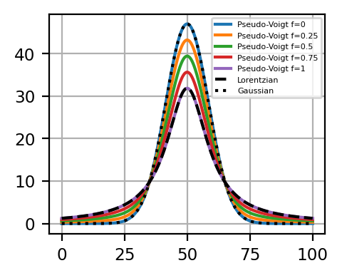
Fig. 7.4 The Pseudo-Voigt Function - The Fraction Parameter

7.1.4. Damped Harmonic Oscillator (DHO)

The damped harmonic oscillator (DHO) describes the power spectrum of density fluctuations of a simple viscoelastic model and is hence commonly used to analyze Brillouin spectroscopic data (Bottani 2018).

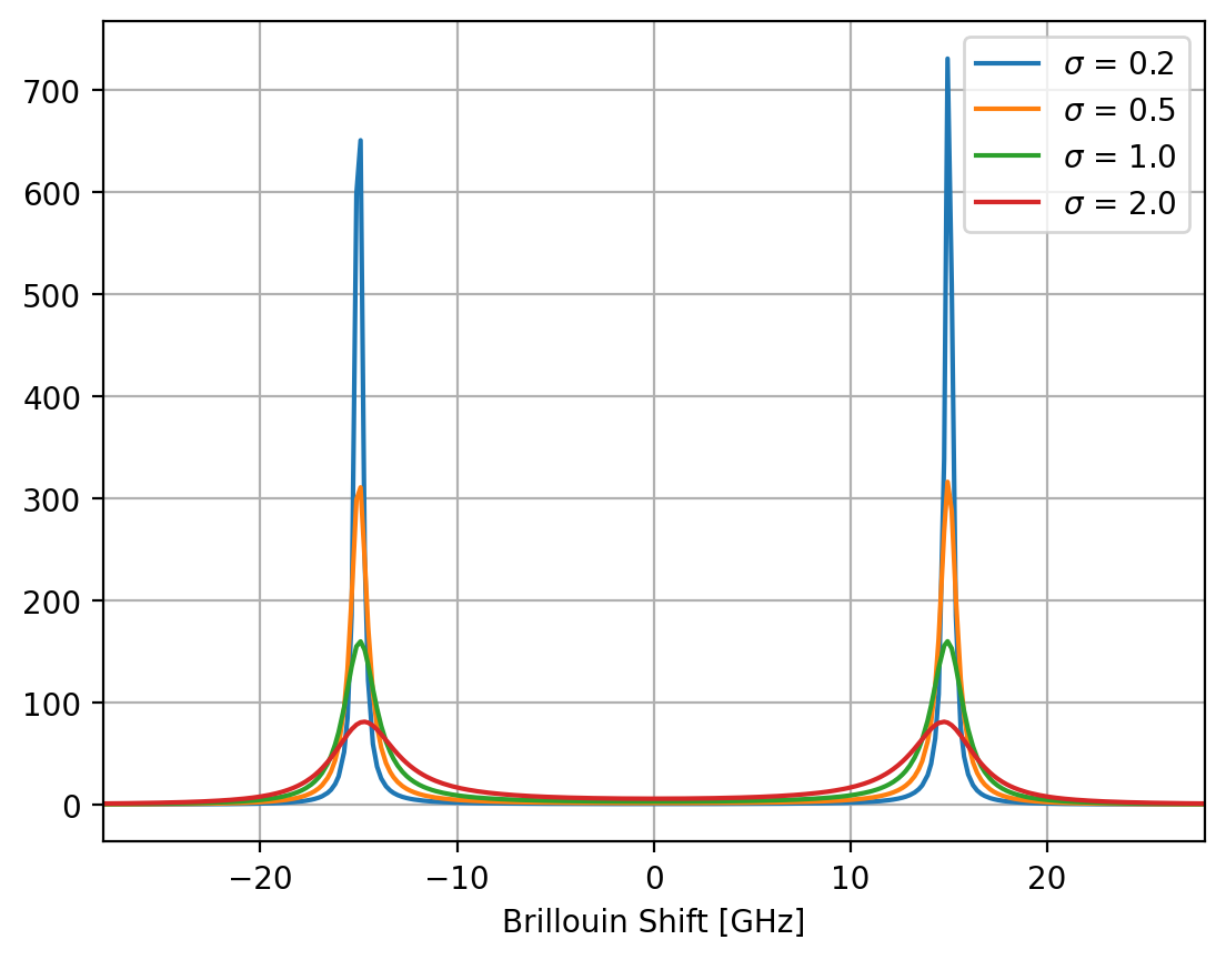
Fig. 7.5 A DHO peak doublet (7.4) for \(A\) = 1000, \(\mu\) = 15 GHz and various values of \(\sigma\).

(7.4)\[ f(x) = \frac{A}{\pi} \frac{2\sigma \mu^2 }{\left( x^2 - \mu^2\right)^2 + \left( 2\sigma x\right)^2} \]

Here, \(2\sigma\) is the full-width at half maximum (FWHM) of the distribution. The square term in the denominator results in an asymmetric line shape that is symmetric about the y-axis (Figure 7.5). The DHO parameters are related to the complex longitudinal elastic modulus \(\hat{M}(x) = M'(x) + i M''(x)\), via \(M'(x) = \frac{\rho}{q^2}\mu^2\) and \(M''(x) = \frac{\rho}{q^2} 2\sigma \mu\), where \(\rho\) is the mass density of the material and \(q\) is the scattering vector \(q = \frac{4 \pi n}{\lambda}\) (Palombo 2019).

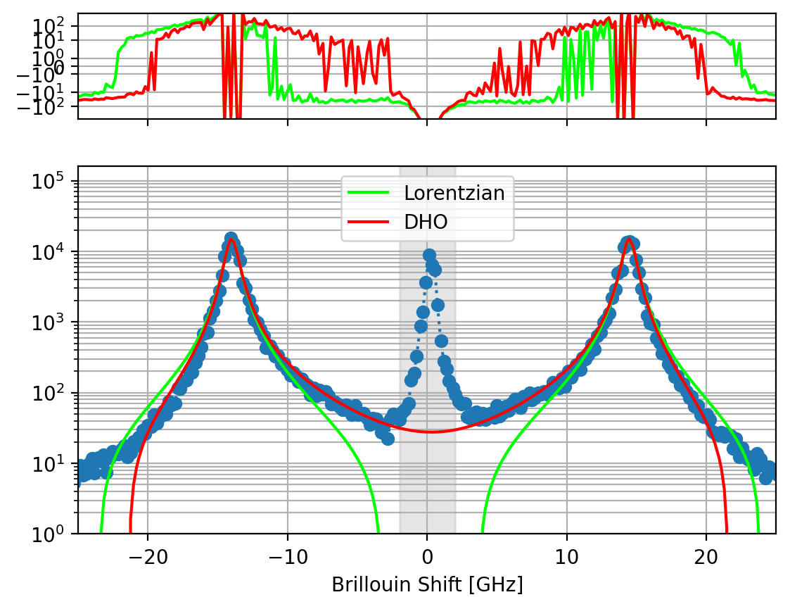
Fig. 7.6 Comparison between DHO and Lorentizan line shapes for a Brillouin scattering spectrum. The grey boxed region has been masked for fitting. The top panel shows the residuals of the fit.

The asymmetric DHO function provides a better fit to Brillouin scattering data than a pair of Lorentzians (Figure 7.6). It is important to note that due to the asymmetry, the parameter \(\mu\) does not correspond exactly to the maximum of the Brillouin peak. Furthermore, the centrosymmetry provides the advantage of fitting the Stokes and anti-Stokes regions of the spectrum simultaneously, effectively doubling the amount of data available to the fitting algorithm. This is similar to averaging the Stokes and anti-Stokes regions during analysis but benefits from the additional data available during the fit and the smaller fit parameter space, which can speed up the fitting procedure.

Note

The centrosymmetric DHO peak implies that elastic Rayleigh scattering occurs at exactly 0 GHz Brillouin shift. This is tricky to implement in practice (Figure 7.7). To this end, SMDExplorer provides a variant of the DHO line shape that accounts for slight offsets \(x_0\) of the fundamental peak from 0 (7.5).

(7.5)\[ f(x) = \frac{A}{\pi} \frac{2\sigma \mu^2 }{\left[ (x - x_0)^2 - \mu^2\right]^2 + \left[ 2\sigma (x - x_0) \right]^2} \]

Please note that if only one side (Stokes or anti-Stokes) is being analyzed, the conventional DHO line shape (7.4) is more appropriate as the additional \(x_0\) parameter is now colinear with the shift \(\mu\), which makes the fit undetermined. In addition, the centrosymmetry implies identical peak heights (\(A\)) for both the anti-Stokes and Stokes part of the spectrum, which is justified for Brillouin scattering data but makes the DHO line shape inappropriate for analyzing the Stokes and anti-Stokes side of Raman spectra where the intensity varies significantly.

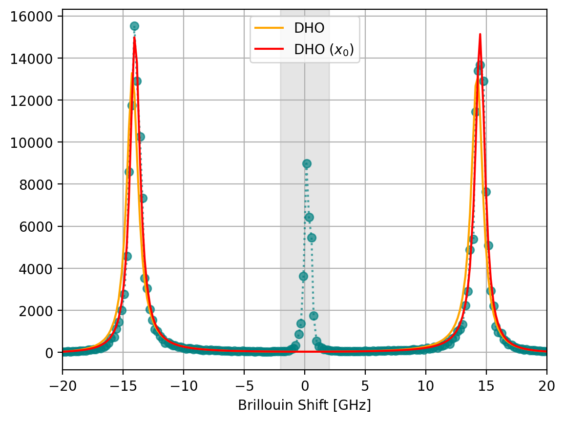
Fig. 7.7 The DHO peak doublet with and without a horizontal offset \(x_0\). While the position of the peaks is similar (14.26 GHz without and 14.27 with offset \(x_0\)), the data’s deviation from centrosymmetry results in an apparent broadening of the peaks (\(\sigma\)=0.575 GHz without and \(\sigma\)=0.498 GHz with offset \(x_0\)).

7.1.5. Which Line Shape Should I Chose?

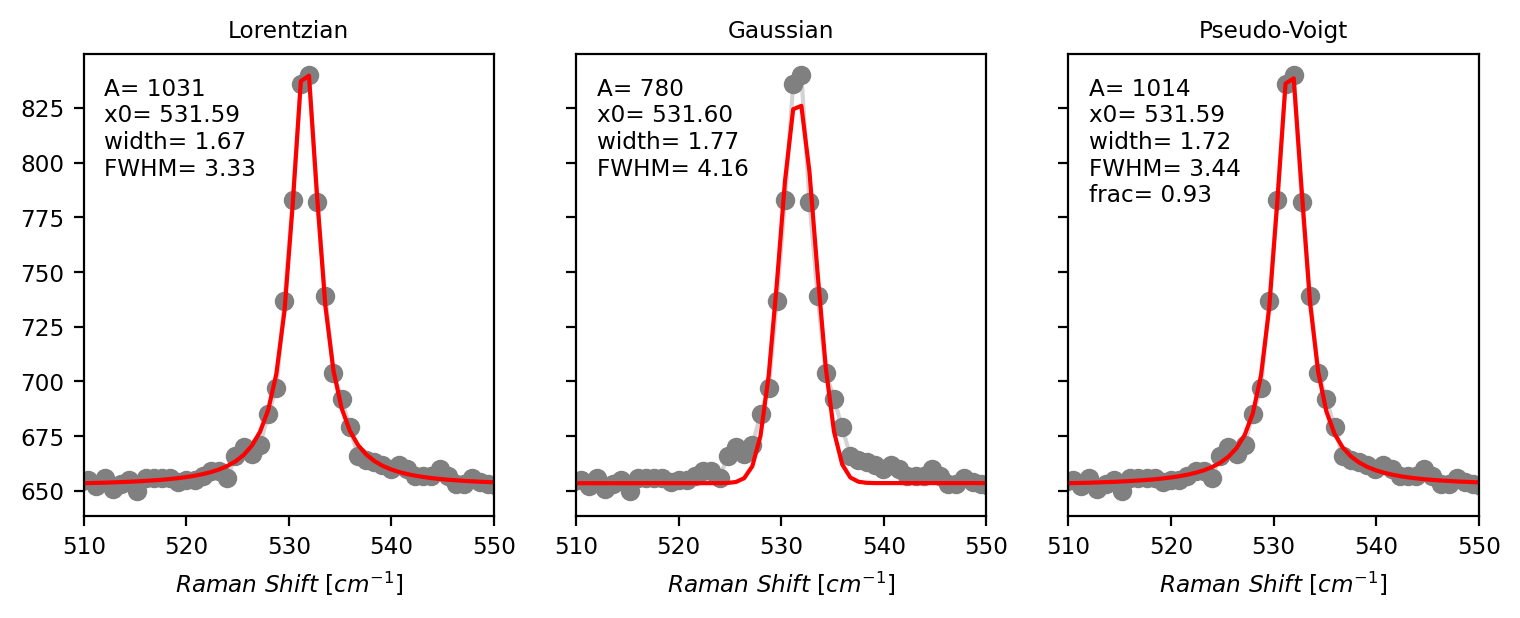
Fig. 7.8 Peak Deconvolution - Line Shape Comparison

The figure Peak Deconvolution - Line Shape Comparison displays the peak deconvolution of a well-isolated single peak in a Raman spectrum with the three line shapes. It is immediately evident that the Gaussian line shape provides the worst fit whereas the Lorentzian and Pseudo-Voigt line shapes match the data closely. In fact, the fraction parameter (\(\alpha\)) of the Pseudo-Voigt peak is close to 1, indicating that this peak is almost purely Lorentzian with only a very minor Gaussian contribution of 7%.

As a starting point, Lorentzian peaks work well for most datasets obtained from Raman or Brillouin scattering. Pseudo-Voigt peaks can be used if the contribution of the (Gaussian) instrument function is significant and the Lorentzian line shape cannot reproduce the experimental data correctly. The additional parameter (fraction \(\alpha\)) leads to a larger parameter space which can make optimization more difficult and slower. If only peak positions are required, any line shape will do essentially (as evident in Peak Deconvolution - Line Shape Comparison), but Lorentzian peaks work tend to work best and are numerically the most simple line shape. DHO peaks are primarily suitable for high-quality Brillouin scattering data where the deviation from the symmetric Lorentzian shape becomes apparent or to take advantage of the combined Stokes and anti-Stokes signal during fitting.

7.2. The Peak Deconvolution Algorithm

SMDExplorer performs peak deconvolution by fitting an experimentally determined spectrum with a sum of peaks, which must all be of the same kind, with an added linear baseline to account for vertical offsets.

(7.6)\[f(x) = y_0 + mx + \sum_i{\frac{A_i}{\pi} \frac{\sigma_i}{(x-\mu_i)^2+\sigma_i^2}}\]

In (7.6), \(y_0\) is the y-intercept of the linear baseline, \(m\) is the slope of the linear baseline, and \(A_i\), \(\mu_i\), and \(\sigma_i\) are the amplitude, position, and width of the i^th Lorentzian peak. The algorithm attempts to minimize the least square error between experimental data (blue trace) and the curve calculated by (7.6), which yields the red trace in Peak Deconvolution - Baseline.

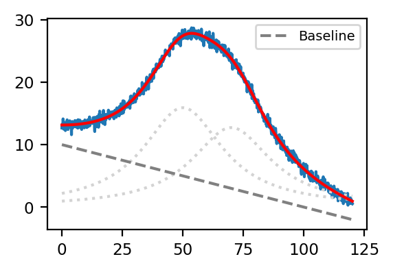
Fig. 7.9 Peak Deconvolution - Baseline

Tip

A linear baseline is often sufficient for peak deconvolution across a small spectral range, even if your data has a non-linear background. If your data has large a non-linear background and you would like to perform peak deconvolution across a wide spectral range, you can subtract the background first using Non-linear Baseline Removal and use the preprocesed, background subtracted data for peak deconvolution.

7.2.1. Initial Guesses

To perform the optimization procedure outlines in The Peak Deconvolution Algorithm, the peak fitting algorithm needs to be supplied with starting values, also known as initial guesses. Good initial guesses are crucial for successful curve fits, in particular during unsupervised fitting of large datasets, where peak positions and amplitude can vary significantly.

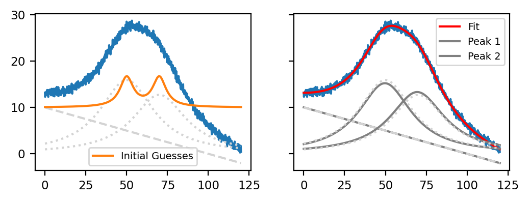
Fig. 7.10 Peak Deconvolution - Good Initial Guesses

The left panel of Peak Deconvolution - Good Initial Guesses displays a synthetic dataset containing two overlapping Lorentzian peaks on top of a linear baseline with some added noise (blue trace). The orange trace in the left panel displays reasonably good initial guesses, and the right panel displays the resulting curve fit that reproduces the original dataset (dashed lines) closely.

Table 7.1 Good Initial Guesses

parameter	value
y0	10
m	0
A1	100
\(\mu\)1	50
\(\sigma\)1	5
A2	100
\(\mu\)2	70
\(\sigma\)2	5

The Table Good Initial Guesses contains the numerical values used for the orange trace in Peak Deconvolution - Good Initial Guesses. It is clear that initial guesses don’t need to be perfect (even though very close initial guesses certainly help), but that the rough peak positions and peak heights should match the original dataset.

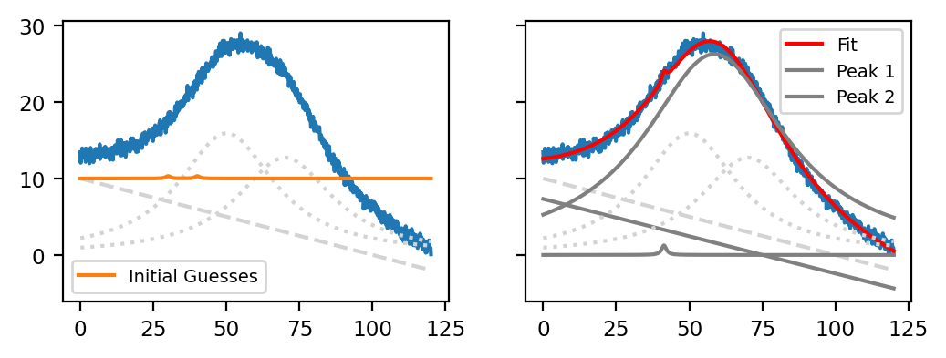
Fig. 7.11 Peak Deconvolution - Bad Initial Guesses

The figure Peak Deconvolution - Bad Initial Guesses shows the same curve fit for another set of (very bad) initial guesses Bad Initial Guesses. While the resulting curve (red trace) actually does match the data (blue trace) fairly well, the red curve only represents one Lorentzian peak on top of the linear baseline while the second peak only has a very low amplitude.

Table 7.2 Bad Initial Guesses

parameter	value
y0	10
m	0
A1	1
\(\mu\)1	30
\(\sigma\)1	1
A2	1
\(\mu\)2	40
\(\sigma\)2	1

Note

The result in Peak Deconvolution - Bad Initial Guesses demonstrates not only how initial guesses affect the outcome of the peak deconvolution procedure but also illustrates that it can be difficult to choose the correct number of peaks. While increasing the number of peaks will generally result in a fit curve that more closely resembles the data - after all there are more parameters for the optimizer to adjust - too many peaks can

• lead to much slower and numerically unstable fits

• result in an underdetermined system where very different parameters can lead to the same result, which makes interpretation difficult. This can (somewhat) be ameliorated by constraints, which will be discussed in the next section

In general, a system with the minimum number of peaks should be prefered. Of course, we know that there are two overlapping peaks present in the example in Peak Deconvolution - Bad Initial Guesses so 2 is the correct number of peaks for modelling this problem.

7.2.2. Constraints

Constraints provide upper and lower limits for the fit parameters and can help the fitting algorithm finding the desired solution. Constraints have two key purposes:

• limiting the parameter space of the fit to physically meaningful values: The amplitude \(A\) and width \(\sigma\) of the line shapes are only meaningful for positive values (or 0), the peak position \(\mu\) should fall within the measure spectral range, and so on.

• steering the fitting algorithm towards the desired solution. This can be relevant in several scenarios:

  • use positional constraints to keep closely-spaced peaks separate

  • use width constraints to prevent overlapping peaks from merging

  • use constraints on the baseline parameters, for example \(m\), to enforce a flat baseline

SMDExplorer offers four different levels of constraining values:

1. no constraints: Constraints are deactivated entirely and fit results can take any value. This is, by far, the fastest option for peak deconvolution.

2. loose constraints: Fit values are not actually constrained (apart from the fraction parameter \(\alpha\) of the Pseudo-Voigt function) but can be adjusted by the user if desired.

3. physical constraints: Here, peak amplitude and width are constrained to positive values.

4. tight constraints: Here, peak amplitude, position, and width are constrained to sensible values for the dataset.

The loose and physical constraint levels are useful starting points for adding user constraints of required. For line shapes other than Pseudo-Voigt, the (unmodified) loose constraint level is functionally equivalent to no constraints at all.

Important

While constraints are important for successful peak deconvolution, especially for automated processing of large datasets where the initial guesses might not be ideal for the entire dataset, constraining the parameter space of the fit coefficients too tightly can significantly slow down the fitting procedure or lead to wrong results entirely. To facilitate chosing suitable constraints, SMDExplorer can display warnings if fit values are being limited by constraints during peak deconvolution and even adjust constraints automatically.

Tip

When to use (or not use) constraints

The fitting algorithm in SMDExplorer is generally quite robust and will, if suitable initial guesses are provided, converge on a reasonable solution even for complex spectra.

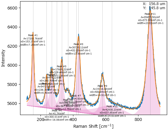
Fig. 7.12 Peak deconvolution on a complex spectrum in SMDExplorer.

For automated peak deconvolution of spectral datasets (spatial or temporal scans, for example), however, applying constrains can be useful and sometimes crucial, particularly if:

• peaks appear or disappear entirely

• the dataset contains strongly overlapping peaks that shift in position (or merge). This is the case in the tutorial dataset.

The first case is illustrated in the waterfall plot below:

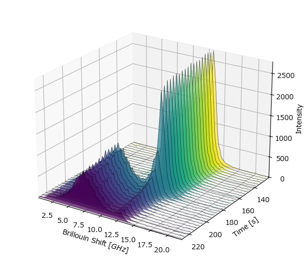
Fig. 7.13 A spectral dataset with a new peak appearing.

Here, a new peak appears at around 180 s. Fitting this dataset with two peaks results in non-sensical (negative) values for the range of the dataset where only one peak exists.

Start

Transition

End

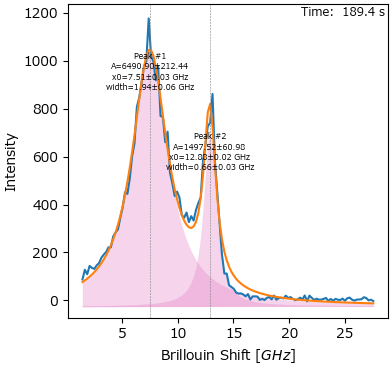
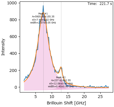
Fig. 7.14 Fitting a dataset with an appearing peak.

Constraining the peak width and height to positive values will simply result in a zero amplitude for spectra where the left peak does not exist yet.

Important

Fitting without constraints is significantly faster than constrained fitting, so, especially for large datasets, constraints should only be used if required. Constraints can be deactivated using the Use Constraints checkbox. See the discussion on how to speed up peak deconvolution for additional tips and tricks.

7.2.3. Masking

Masking allows excluding a spectral range from the fit. The masked area is not taken into account when comparing the calculated fit curve with the original spectrum, thus allowing large deviations between the two in the masked region. This is useful when performing peak deconvolution on both the Stokes and anti-Stokes region in Brillouin or Raman spectroscopy where the central Rayleigh peak often has much higher intensity then the actual signal.

Note

Regions at the left or right edges of the spectrum can be excluded by Range Selection. Masking is for removing parts of the spectrum that are at the center of the range of interest.

See also

Spectral regions can also be masked using the Range Selection preprocessing step. In this case, the masked region is replaced by a straight line connecting the start and end point. Both types of masking may be used in combination.

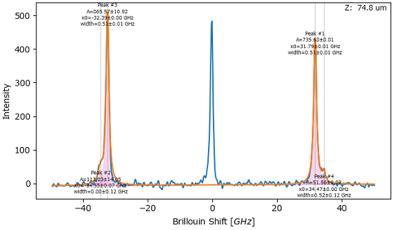
Fig. 7.15 Peak Deconvolution - Masking

Important

Masking of the fundamental is crucial when using the DHO line shape to fit the Stokes and anti-Stokes side of a Brillouin spectrum simultaneously.

7.2.4. GPU-accelerated Fits

SMDExplorer allows peak deconvolution to be performed on the machines GPU, which can lead to significant faster fits for datasets with a large numbers of spectra or many fit parameters (Figure 7.16). The GPU-based fit functions (e.g. Lorentzian (GPU)) are identical to the CPU-based equations. GPU-based fitting is enabled if the following conditions are met:

• the platform is Windows or Linux

• a CUDA-enabled GPU is installed

• the CUDA version is 12 or higher. The supported CUDA version is tied to the installed GPU driver.

  Hint

  The CUDA version can be checked by entering nvidia-smi in the command line.

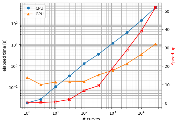
Fig. 7.16 Runtime comparison of GPU (RTX 3050 Laptop) and CPU (Core i7, single threaded) fits.

7.3. The Fitting Window

The Fitting Window contains the user interface to guide you through the process of peak deconvolution for a single spectrum or a multi-spectrum dataset. The window is divided into four panes:

• the top Settings pane (green box in Peak Deconvolution - The Fitting Window) contains the controls for calculating initial guesses, masking, selecting a line shape, and ultimately performing the curve fit.

• the Fit Coefficients pane (blue box in Peak Deconvolution - The Fitting Window) contains the numerical values of the fit parameters as well as their constraints.

• the Fit Result pane (red box in Peak Deconvolution - The Fitting Window) contains the graphical representation of the fit parameters in the the Fit Coefficients pane

• (multi-spectral scans only) the Trace Selection pane (orange box in Peak Deconvolution - The Fitting Window) contains a mapping / intensity profile of the entire dataset. Clicking or dragging in the Trace Selection pane updates the spectrum displayed in the Fit Result pane.

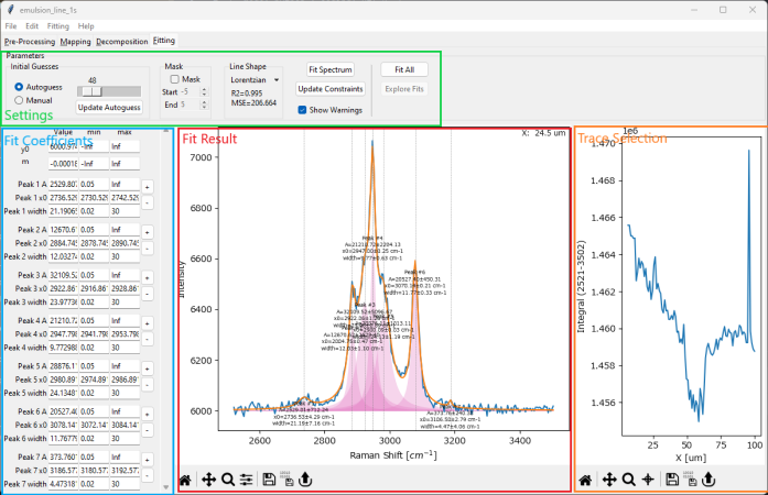
Fig. 7.17 Peak Deconvolution - The Fitting Window

7.3.1. The Settings Pane

The Settings pane contains the controls to configure and initiate the peak deconvolution procedure.

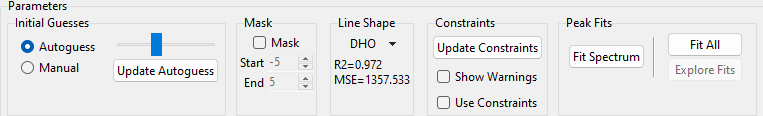
Fig. 7.18 Peak Deconvolution - The Settings Pane

The controls are (from left to right):

1. the Initial Guesses section. This section controls computation of initial guesses. Initial guesses can be entered in in two ways:

   Autoguess

   This mode is selected using the Autoguess radio button and tries to compute initial guesses by detecting peaks in the spectrum. Peak detection sensitivity can be adjusted using the slider: Moving the slider to the right decreases the sensitivity, resulting in fewer detected peaks, moving the slider to the left increases sensitivity, detecting smaller or more overlapping peaks. The Fit Result pane will update automatically when the slider is moved, which provides graphical feedback on the found peaks.

   Note

   The Autoguess slider adjusts peak prominence, which is the distance the a peak rises over the surrounding spectrum. Increasing the threshold prominence (moving the Autoguess slider to the right) requires a higher distance between the top of the peak and the next adjacent minimum. The peak detection algorithm works on the preprocessed data and can thus be affected by noise. In addition, strongly overlapping peaks with no trough inbetween will likely be missed by this approach. In this case, peaks can be added or removed manually.

   Tip

   If there is little effect when moving the Autoguess slider, try clicking the Update Autoguess button. This will recalculate the lower and upper boundary of the slider for the spectrum currently displayed in the Fit Result pane.

   Manual

   This mode is selected using the Manual radio button. Clicking the Enter Positions button displays a prompt to enter peak positions.

   Hint

   The Fit Coefficients Pane also allows addition and deletion of peaks as well as adjusting all peak and baseline coefficients. Using the Autoguess mode followed by manual adjustment of peak number and parameters is generally the fastest way to get good initial guesses.

2. the Mask section. Here, you can exclude a spectral region at the center of the currently selected range from the peak deconvolution procedure.

   Mask

   Turns masking on or off.

   Start

   The beginning of the masked spectral range

   End

   The end of the masked spectral range

3. The Line Shape section allows you to select a line shape. Currently supported line shapes are

   • Gaussian

   • Lorentzian

   • Pseudo-Voigt

   • Damped Harmonic Oscillator (DHO), including the DHO (x₀) variant

   After performing a fit, the Line Shape section will also display the mean squared error (MSE) and the R² score of the currently displayed spectrum and the current fit curve.

4. The Constraint section controls if and how constraints are applied during the fit.

   Update Constraints

   Clicking this button will update the position constraints \(\mu_{min}\) and \(\mu_{max}\) of all peaks to that the current position \(\mu\) is at the center of the range \([\mu_{min} ... \mu_{max}]\). The span of the range (\((\mu_{max} - \mu_{max}) / {2}\)) can be adjusted in Preferences.

   Use Constraints

   Activates or deactivates constraints during the fit. Constraining peak positions or widths helps steering the fitting algorithm to physically meaningful solutions but can significantly slow down the fitting procedure. For a detailed discussion on the merits and disadvantages of constraints, see the section Constraints. Right clicking on the Use Constraints check box allows switching between different levels of default constraints.

   Show Warnings

   Display a warning message if a fit parameter is being limited by the currently set constraints.

5. The Fit section contains the controls for performing peak deconvolution on the currently displayed spectrum.

   Fit Spectrum

   Performs peak deconvolution on the currently displayed spectrum using the parameters in the Coefficient Pane as starting values. After a successful fit, the computed curve in The Fit Result Pane as well as the values in the Coefficient Pane will be updated to reflect the optimized values found during the fitting procedure.

6. (multi-spectral scans only) The Analyze Dataset section. Here, you can perform peak deconvolution on a large spectral dataset, e.g. a spatial or temporal scan.

   Fit All

   Fits all spectra in the dataset displayed in the Trace Selection pane using the values displayed in the Coefficient Pane as starting values. After fitting is complete, selecting a spectrum from in the Trace Selection pane displays the spectrum along with the fit result in the The Fit Result Pane.

   Important

   Good initial guesses and, if applicable, constraints are crucial for performing successful automated peak deconvolution on large datasets, especially if peak intensities or position vary greatly. It is advisable to verify that the current set of parameters works for the entire dataset by selecting a few spectra and performing a single spectrum fit before trying to fit the enture dataset at once.

   Warning

   Depending on the size of your dataset, peak deconvolution may take a long time. SMDExplorer uses multi-threading for large datasets / many peaks to speed up fitting. Multi-threading parameters can be configured in Preferences. See the section on how to speed up peak deconvolution for additional tips and tricks.

   Explore Fits

   This option becomes available after performing peak deconvolution on a dataset. Clicking the Explore Fits button opens the Peak Deconvolution Analysis window to visualize and analyze the peak deconvolution result.

7.3.2. The Fit Coefficients Pane

The Fit Coefficients pane contains the numerical values of the parameters of the fit curve displayed in The Fit Result Pane as well as their upper and lower limits.

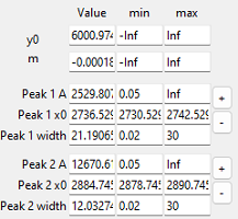
Fig. 7.19 Peak Deconvolution - The Fit Coefficients Pane

The pane is divided into four columns. The first column contains an identifier for the parameter in this row. The parameters \(\rm{y_0}\) and \(\rm{m}\) are the y intercept and slope of the linear baseline, Peak 1 \(\rm{A}\) is the amplitude of peak 1, Peak 1 \(\rm{x_0}\) the position of peak 1, Peak 1 \(\rm{width}\) the width of peak 1, and so on. The next two columns contain the lower and upper limits, with Inf indicating infinity (\(+\infty\)) and -Inf indicating negative infinity (\(-\infty\)). Setting the upper and lower bounds to ±Inf means that this parameter is unconstrained and can take any value.

The last column contains a + and - button.

+

Adds a peak after the selected peak. You will be prompted to enter a peak position for the new peak. Width and amplitude of the new peak as well as suitable constraints will be computed automatically.

-

Deletes the selected peak.

To adjust initial guesses or constraints simply enter a new value into the field of the parameter you would like to adjust. The calculated fit curve in Peak Deconvolution - The Fit Result Pane will adjust accordingly.

Note

SMDExplorer will perform sanity checks on initial guesses and constraints to make sure that fitting is feasable with the new parameter. If the new parameter is infeasible, a warning will be displayed.
Positional constraints will be adjusted automatically to flank the newly entered position.

Tip

After performing a fit, the optimized fit parameters will be displayed in The Fit Coefficients Pane. The entire set of values can be copied to the clipboard by right-clicking on the Fit Coefficients pane and selecting Copy from the context menu or by standard keyboard shortcuts when the Fit Coefficients pane has focus.

This exports the data in the form

parameter	value	uncertainty
y0	5803.4563	2.840
m	-0.00027	0.000818
Peak_1_A	7104.49	2194.39
…	…	…

where the uncertainties are the one standard deviation errors of the parameters.

7.3.3. The Fit Result Pane

The Fit Result Pane displays the currently selected spectrum (blue trace) as well as the fit curve calculated from the parameter set in The Fit Coefficients Pane (orange trace). In addition, the graph contains indicators of peak positions (gray vertical lines), a curves of the individual peaks (pink) and, for each peak, information about the peak parameters. Display of peak parameter information can be turned on or off by the Fitting ‣ Show Peak Info menu item. Display of the pink peak curves can be toggled by the Fitting ‣ Show Peaks menu item.

Note

Before performing a fit, the peak information text contains the values of the initial guesses. After fitting, the peak information will contain the optimized parameters and their uncertainties (± one standard deviation).

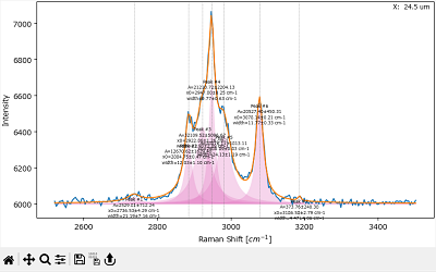
Fig. 7.20 Peak Deconvolution - The Fit Result Pane

7.4. Peak Deconvolution - A How-to

This section provides instructions for performing peak deconvolution for a dataset containing multiple overlapping peaks.

• Preprocessing

  • (optional) spectral Calibration. This is particularly relevant if peak peak deconvolution is performed to extract absolute peak positions.

  • Range Selection. Peak deconvolution is performed on the entire spectral range of the raw or preprocessed dataset so range selection is required to define a spectral range of interest. Regions at the center of the selected range of interest can be excluded using masking.

  • (optional) Cosmic Ray Removal (Despiking). If your dataset contains cosmic ray artifacts in the range of interest, despiking is recommended before peak deconvolution

  • (optional) Non-linear Baseline Removal. The linear baseline of the peak deconvolution algorithm is typically sufficient when the curvature of the baseline is not too high. If a linear baseline is insufficient, in particular when the selected range is large, you can perform non-linear baseline subtraction.

  • (optional) Averaging / Binning / Denoising or Smoothing. Peak deconvolution is, in general, not very sensitive towards noise and care should be taken to avoid spectral distortion by smoothing or denoising.

  • (optional) Normalization. Normalization can be useful to counter the effects of focal drift. Alternatively, the ration of peak amplitudes can be analyzed in the Peak Deconvolution Analysis window.

  • (optional) Masking. The Masking preprocessing step excludes entire spectra from further analysis based on their spectral intensity. This can be useful to remove, for example, empty spectra from peak deconvolution.

  Apart from Range Selection to select the spectral range of interest to be fit, all preprocessing steps are optional and should be used judiciously.

• To perform peak deconvolution, apply the selected preprocessing steps and switch to the Fitting window. The following steps provide an outline on how to find initial guesses, optimize the number of peaks, their parameters and constraints, and perform the fit.

  1. (multispectral datasets) select a representative spectrum by clicking and dragging in the Trace Selection pane.

  2. Click the Update Autoguess button and adjust the sensitivity slider to detect peaks. This will update the graph in the Fit Result pane. Peak widths and amplitudes will likely not match the peak shape of your dataset yet. This will be addressed in the next step.

     Tip

     Move the peak sensitivity slider to find peaks approximately in the right places. Peaks can always be added or removed manually later on. It is likely that automatic peak detection will fail to detect strongly overlapping peaks as separate peaks.

     

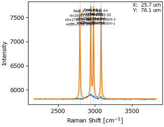
     Fig. 7.21 Approximate Peak Detection

  3. Click the Fit Spectrum button to optimize the set of initial guesses. The graph in the Fit Result pane will be updated to allow judging whether the number of peaks as well as their positions in the set of initial guesses were sufficient to reproduce the spectrum.

  

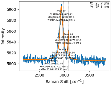
  Fig. 7.22 Initial Optimization

  4. Add or remove peaks if required using the Fit Coefficients pane. Click the Fit Spectrum button to update the resulting fit curve.

  5. (optional) Optimize fit parameters if constraints are activated.

     • manually adjust peak positions and constraints in the Fit Coefficients pane or

     • click the Update Constraints button to adjust all constraints

     Click Fit Spectrum to update the result. Generally, several rounds of Update Constraints and Fit Spectrum can help to find suitable initial positions and positional constraints. Alternatively, an unconstrained fit can be performed be deactivating the Use Constraints checkbox, followed by reactivating constraints and clicking Update Constraints to update the constraints to the new positions.

  

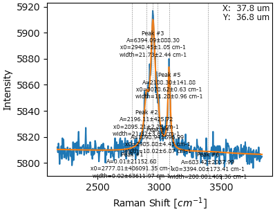
  Fig. 7.23 The optimized parameter set (number of peaks, peak parameters, constraints)

  6. (multispectral datasets) select a different spectrum from the dataset and check whether the number of peaks and their parameters can successfully fit the new spectrum. Adjust and optimize parameters as outlined above.

  7. (optional) activate the Show Warnings checkbox and click the Fit Spectrum button. If fit parameters are being limited by their constraints, a warning will be shown to identify the issue.

     Note

     Depending on the dataset, limiting parameters by constraints is unavoidable or even desired to prevent, for example, closely spaced peaks from merging. The Show Warnings option is merely a debugging tool to help identify unsuitable constraints, particularly for datasets with many peaks where issues are not immediately apparent.

     Hint

     If you find the default limits on peak position and width too restrictive, you can adjust these values in Preferences.

  8. (multispectral datasets) Click the Fit All button to perform peak deconvolution on the entire dataset. Once the entire dataset has been processed, you can inspect the fit result for each spectrum by clicking and dragging in the Trace Selection pane.

  9. (multispectral datasets) Analyze the peak deconvolution result.

  10. (multispectral datasets, optional) Save the fit result using Fitting ‣ Save Fit Result. The saved fit result can be imported using Fitting ‣ Load Fit Result.

      Important

      Please be aware that a loaded fit result might not match the loaded data if data preprocessing is different. For best results, save the preprocessed data along with the fit result using File ‣ Save Preprocessed Data

Tip

Peak deconvolution of large datasets can potentially take a long time. Here are several hints how to speed up procesing:

• Reducing the number of points by range selection. The lower the number of points, the faster the fit.

• Reducing the number of peaks. While SMDExplorer excels at peak deconvolution of complex spectra, it can be significantly faster to fit different spectral regions independently. The can (again) be achieved using range selection.

• Excluding atypical spectra by masking.

• Deactivating constraints if possible.

• Using suitable initial guesses.

• Optimizing the multithreading settings for your machine.

7.5. Analyzing and Visualizing Peak Deconvolution Results

The Peak Deconvolution Analysis Window allows the analysis of peak deconvolution results

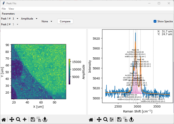
Fig. 7.24 The Peak Deconvolution Analysis Window

Parameters

Peak 1#

Selects a a peak for analysis. The numbering is the same as in the Fit Coefficients Pane. Peak numbers also will be displayed in the Fit Result pane if Show Spectra is selected.

Note

Peak numbering is not neccessarily ordered by peak position.

Peak Parameter

Selects which parameter of the selected peak to analyze. Parameters are:

• peak amplitude

• peak position

• peak width

• peak FWHM

• (for Pseudo-Voigt peaks only) fraction (ration between Gaussian and Lorentzian)

See Anatomy of a Peak for a discussion of the parameters and the description of the line shapes for the exact definition.

Selecting a Peak 1# and a Peak Parameter will update the Fit Result Mapping displayed in the left pane of The Peak Deconvolution Analysis Window.

Operation

Performs an arithmetic operations on the selected parameter of one or two selected peaks

• None: No operation. Plots the selected parameter of the selected peak

• Ratio: Plots the ration (quotient) of the selected parameter of the first peak and the same parameter of the selected second peak.

• Average: Plots the average (arithmetic mean) of the selected parameter of the first peak and the same parameter of the selected second peak.

• Abs. Average: Plots the average (arithmetic mean) of the absolute value of the selected parameter of the first peak and the absolute value of the same parameter of the selected second peak.

  Tip

  This operation is useful for determining average positions when fitting both Stokes and anti-Stokes peaks, which is commonly done in Brillouin spectroscopy.

• Sum: Plots the sum of the selected parameter of the first peak and the same parameter of the selected second peak.

• Abs. Sum: Plots the average sum of the absolute value of the selected parameter of the first peak and the absolute value of the same parameter of the selected second peak.

Peak 2#

Selects a second peak for analysis, for example for plotting amplitude ratios.

Show Spectra

Shows or hides the Fit Result pane. The spectrum and fit result shown in the Fit Result pane can be updated by clicking and dragging on the Fit Result Mapping.

Compare

Opens a Fit Analysis Comparison window or append the current mapping to the already opened Fit Analysis Comparison window. For details, see Comparing Intensity Profiles / Images. For three-dimensional data, a 2D plot will be displayed.

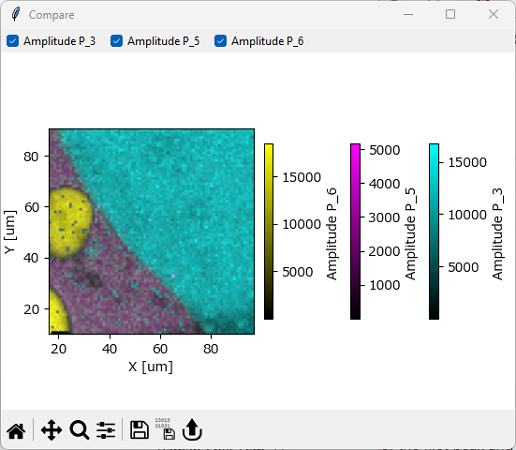
Fig. 7.25 Overlaying Fit Analysis Results

For two-dimensional data, Line Profile Analysis is available via View ‣ Line Profile.
In addition, an amplitude mask can be applied to the displayed mapping using View ‣ Use Amplitude Mask. This allows excluding datapoints where a selected peak has an amplitude below a certain threshold from display.

See also

Low-intensity (or empty) spectra can also be excluded from analysis using Masking. Removing these spectra before fitting has the additional benefit to speed up data processing.

The Peak Deconvolution Analysis Window allows export of peak fitting results as .hdf5 or .csv files using File ‣ Save Fitting Result. When exported as .hdf5, peak fit data can be re-imported into SMDExplorer. See HDF5 Peak Fitting Results for the .hdf5 specification.