8. Particle Analysis#
Particle analysis allows the computation of image metrics of using images obtained from two-dimensional spectral mappings, e.g. using manual or automated image formation. Particle analysis can be accessed via the right-click context menu in all two-dimensional spectral mappings.
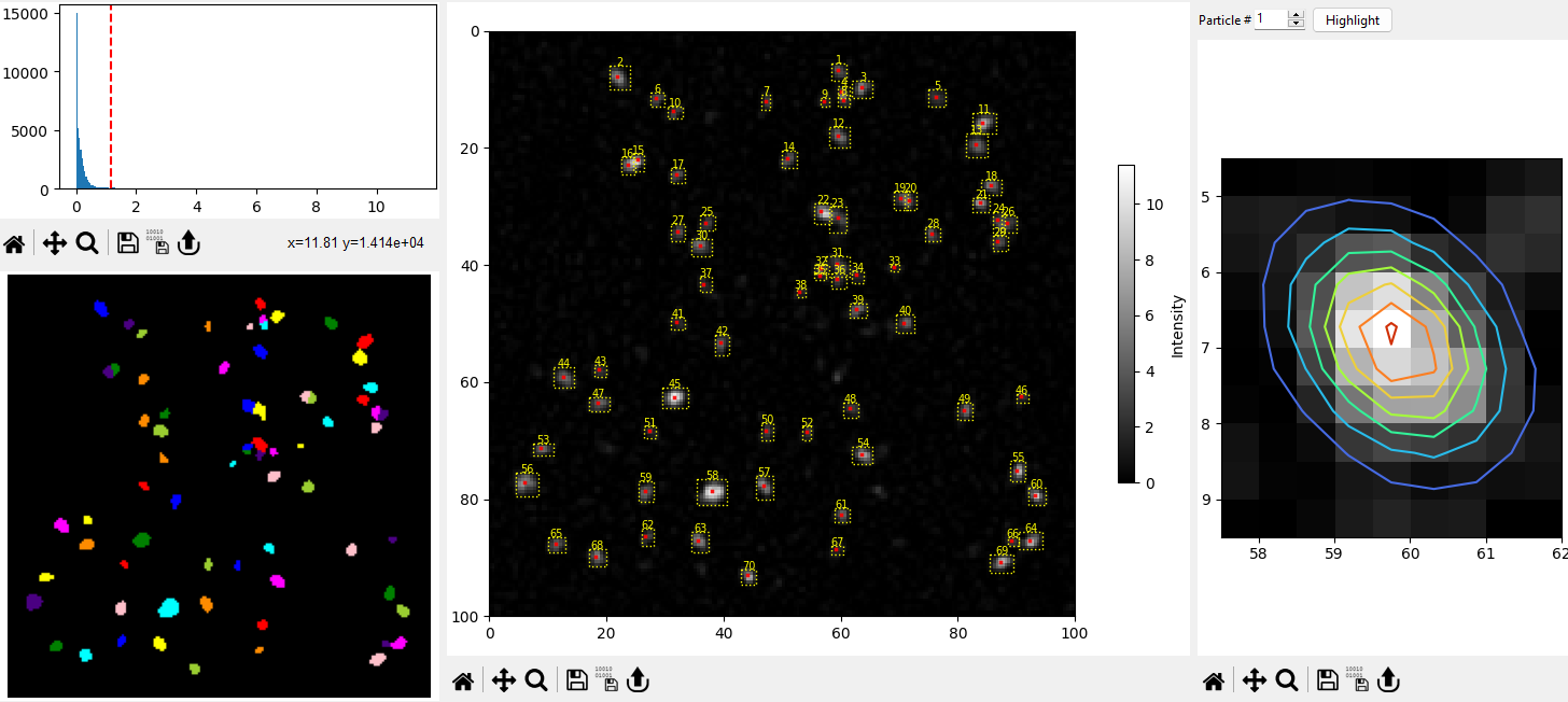
Fig. 8.1 Particle Analysis#
Particle analysis allows the identification or particles (i.e. bright spots) in an image, e.g. a spectroscopic mapping. Various parameters of the identified particles (location, average and maximum brightness, area) can be computed.
Note
Particle analysis assumes bright particles on a dark background.
8.1. The Particle Analysis Window#
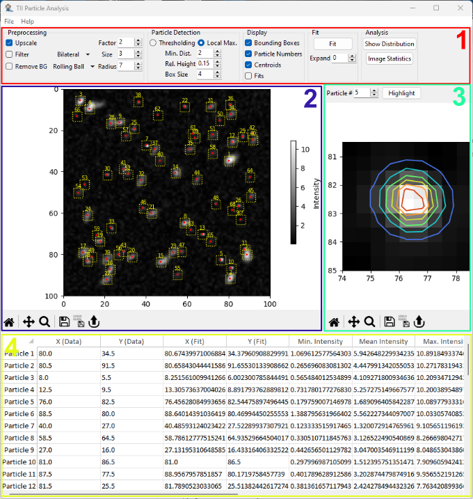
Fig. 8.2 The Particle Analysis Window#
The user interface of the particle analysis window consist of several subwindows:
The Parameter Toolbar, which controls image preprocessing, particle detection, particle display, fitting, and analysis.
The Image Pane, which contains the image being analyzed. Detected particle parameters, i.e. bounding boxes and centroids, can be displayed here a well.
The Particle Detail View, which contains the cropped image of a single particle as well as the contour plot of a two-dimensional Gaussian fit if fitting has been performed.
The Results Table, which displays the numerical values of the parameters extracted from the detected particles.
8.1.1. The Parameter Toolbar#
The Parameter Toolbar controls processing, analysis, and display parameters.
8.1.1.1. Preprocessing#
Preprocessing allows modification of the image of interest prior to particle detection and analysis.
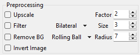
Fig. 8.3 Preprocessing Controls#
- Upscale
Upscales (zooms) the image by
Factor.- Filter
Removes noise from the image by applying a filter. Available filters are:
Gauss: a Gaussian blur filter
Bilateral: An edge-preserving denoising filter that averages pixels based on their proximity and similarity
Total Variation: An edge-preserving denoising filter that averages similar regions in an image.
The filter
Sizecontrols the size of the window over which pixels are averaged. A higher value removes more noise but results in a blurrier image.
- Remove BG
Activates background removal using the Rolling Ball method, which is essentially a spatial high-pass filter. The
Radiusparameter controls the size of the filter, which should (roughly) be equal to or smaller than the curvature of the non-homogeneous background.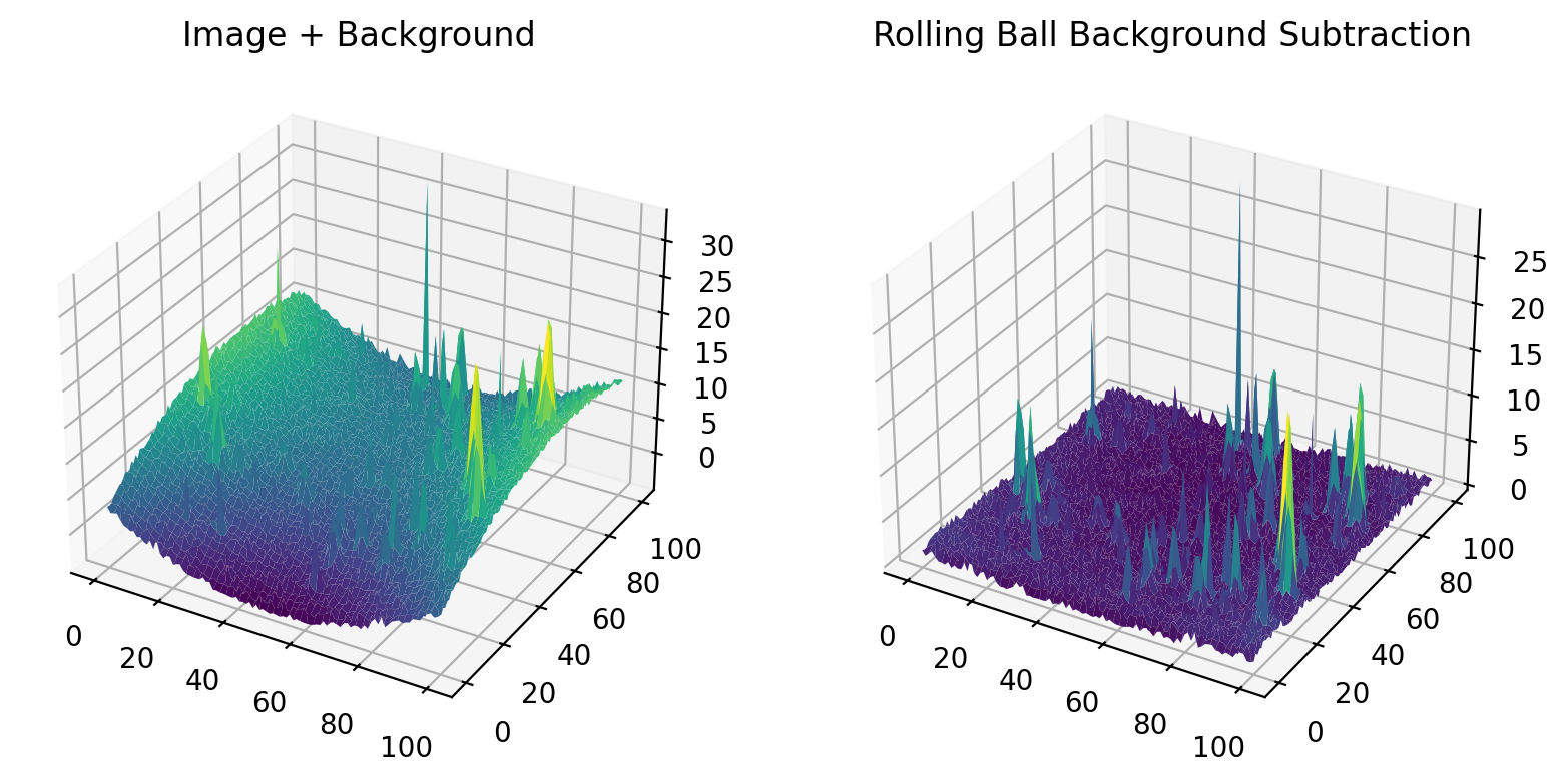
Fig. 8.4 Rolling Ball Background Subtraction#
Note
Rolling Ball background subtraction assumes bright particles on a dark background.
- Invert
Inverts the image. Use this if your data consists of dark particles on a bright background. This processing step is always performed first.
The Image Pane provides immediate visual feedback on the activated preprocessing steps and the selected parameters.
8.1.1.2. Particle Detection#
Particle detection can be performed using two methods:
Local Maxima Detection: Here, particles are identified as the local maxima in a sliding window. This method is useful for speckle images. Particles are assumed to be Gaussian blobs.
Thresholding. Here, particles are identified as regions brighter than the background intensity (threshold). No assumption about the particle shape is made but it can be difficult to identify particles with drastically different brightness.
8.1.1.2.1. Local Maxima Detection#
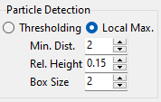
Fig. 8.5 Local Maximum Particle Detection Parameters#
Particle detection can be adjusted using the following parameters:
- Minimum Distance
The minimum separation between particles. Particles are the local maxima in the region \(2 \cdot d_{min} +1\). This value is in pixel and should be adjusted depending on image size and particle density.
- Relative Height
The minimum relative intensity of the particle, as a fraction of the maximum image intensity.
- Box Size
The size of the bounding box around the particle center (in pixel). The bounding box is drawn in the region \([-d_{box}, +d_{box}+1]\), meaning a box size of 2 results in a bounding box of 5 pixels (width and height).
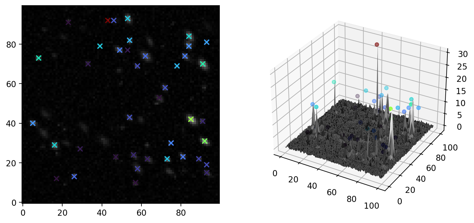
Fig. 8.6 Local Maximum Particle Detection#
The Image Pane provides immediate visual feedback on the selected parameters.
8.1.1.2.2. Thresholding#
In Thresholding mode, particles are identified as bright, contiguous areas with an intensity above a threshold. Thresholding parameters can be adjusted in the thresholding parameters section of the toolbar. When switching to thresholding mode, the thresholding pane is inserted on the left side of the image pane to provide additional visual feedback of the thresholding parameters and the detected particles.
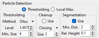
Fig. 8.7 Thresholding Particle Detection Parameters#
- Level
The intensity threshold. The default value is computed using Otsu’s Method. Pixels with an intensity lower than level are considered background, pixels brighter than the threshold are considered part of a particle. The threshold can be adjusted using the Level spinbox or by dragging the red vertical line in the image intensity histogram (top panel in the thresholding pane).
- Minimum Size
The minimum size of the detected particles (in pixel)
- Cleanup
Removes spurious, small particles and closes holes in otherwise contiguous particle regions using morphological operations on the binarized image. Methods are:
The size parameter determines the size of the square morphological element.
- Segmentation
Attempts to split merged blobs into separate particles based on watershedding.
- Minimum Distance
The minimum distance between sub-particles (in pixels)
- Relative Height
The minimum relative intensity of the particle, as a fraction of the maximum image intensity.
Note
Particles are identified by different colors in the bottom image of the thresholding pane. This allows visual confirmation of successful particle segmentation.
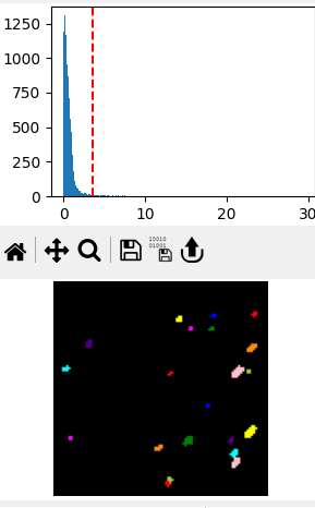
Fig. 8.8 The Thresholding pane#
Detected particles are displayed in different colors at the bottom of the thresholding pane.
In addition Image Pane provides immediate visual feedback on the selected parameters.
8.1.1.3. Display#
The Display section of the toolbar controls which particle parameters are displayed in the image pane.
Note
Fit contour plots will only be displayed if fits have been performed. Any change in particle detection or preprocessing parameters will invalidate the fit results.
8.1.1.4. Fit#
The Fit section of the toolbar allows fitting a bivariate (two-dimensional) Gaussian distribution to each particle. This is particularly useful for speckle images where the detected particles have (approximately) elliptical shapes. The two-dimensional Gaussian function is given by (8.1).
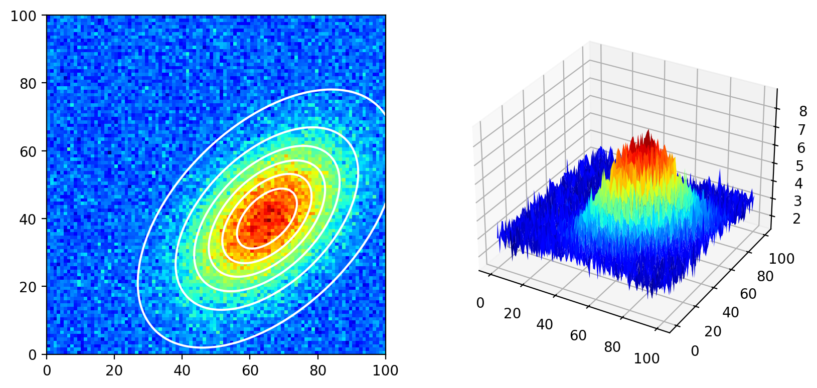
Fig. 8.9 A bivariate Gaussian distribution.#
Here:
\(z_0\) is the vertical offset of the Gaussian
\(A\) is the amplitude (height) of the Gaussian
\(x_0\) and \(y_0\) are the horizontal and vertical centers of the Gaussian peak
\(\sigma_x\) and \(\sigma_y\) are the horizontal and vertical widths of the Gaussian (standard deviation)
\(\xi\) is a correlation parameter between the horizontal and vertical width. The effect of the correlation parameter \(\xi\) is shown below.
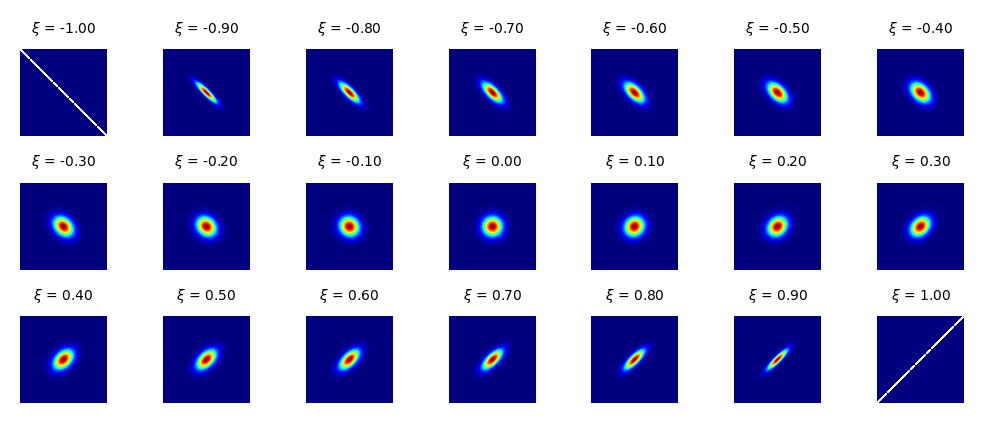
Fig. 8.10 The correlation parameter \(\xi\).#
Fits are calculated after pressing the Fit button. A contour plot of the calculated Gaussian function will be displayed in the particle detail view and (optionally) in the image pane and fit results will be appended to the results table.
- Expand
Expands the bounding box of the particle by the selected number of pixels before performing the fit. This is useful for particles detected by Thresholding, where the bounding box is the smallest rectangle that encloses the particle. This bounding box is often too tight to provide a sufficient number of baseline data to perform a successful fit. Fit particles detected using Local Maximum Detection, the Expand parameter has the same effect as a manual increase in bounding box size.
Important
A higher number of datapoints generally improves fit convergence. This can be achieved by
increasing the image region around the particle that is used for the fit (using Expand or by increasing the particle bounding box).
When increasing the particle bounding box, care should be taken to avoid including nearby particles in the fit region. The region of the image used for the fit is displayed in the particle detail view.
upscaling the image to increase the total number of datapoints.
The minimum number of points required for the fit is the number of fit parameters (7) in (8.1).
8.1.1.5. Analysis#
The Analysis segment of the toolbar gives access to the Parameter Distributions and Image Statistics windows.
8.1.2. The Image Pane#
The image pane displays the selected image as well as (optionally):
particle centroids (centers)
particle bounding boxes
particle numbers
contour plots of two-dimensional Gaussian fits (if fits have been performed).
Display parameters can be toggled in the Display section of the parameter tool bar.
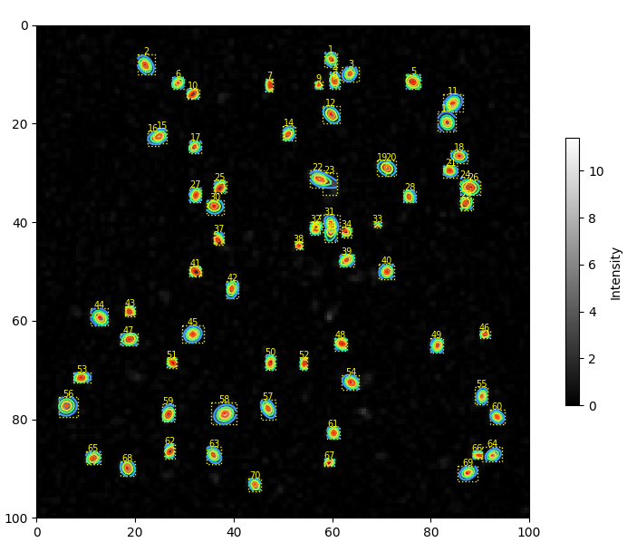
Fig. 8.11 The analyzed image with fits overlayed.#
Tip
Double-clicking on a particle in the image pane will display this particle in the Particle Detail view.
8.1.3. The Particle Detail View#
The particle detail view displays a close-up view of each particle within the border of the particles’s bounding box (optionally expanded by the Expand factor). If fits have been performed, a contour plot of the two-dimensional Gaussian function ((8.1)) is displayed as well. The Highlight button highlight the selected particle in the main image pane.
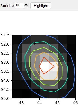
Fig. 8.12 The Particle Detail View.#
8.1.4. The Results Table#
The Results Table contains the numerical values of the particle analysis. Available parameters are:
X (Data) & Y (Data): The position of the centroid of the detected particle (in image coordinates).
Min. Intensity (Region): The minimum intensity in the particle bounding box, in other words the background intensity in the vicinity of the particle.
Mean Intensity: The mean intensity of the particle.
Max. Intensity: The maximum intensity of the particle.
Max - Min Intensity: The height of the particle (max. intensity - baseline).
(thresholding only) Area (Particle): The area of the particle in image units.
(thresholding only) Min Intensity (Particle): The minimum of the particle.
If fits have been performed, the following additional parameters are available.
X (Fit) & Y (Fit): The position of the center of the two-dimensional Gaussian distribution (\(x_0\) and \(y_0\) in (8.1)) in image coordinates.
Z0 (Fit): The baseline offset of the Gaussian distribution (\(z_0\) in (8.1)).
A (Fit): The baseline amplitude of the Gaussian distribution (\(A\) in (8.1)).
Sigma X (Fit) & Sigma Y (Fit): The widths (standard deviations) of the Gaussian distribution (\(\sigma_x\) and \(\sigma_y\) in (8.1)).
Xi (Fit): The correlation parameter the Gaussian distribution (\(\xi\) in (8.1)).
Area (Fit): The area of an ellipse of the \(2\sigma\) confidence interval. The major and minor semi-diameters \(a\) and \(b\) are the square-roots of the eigenvalues of the covariance matrix \(\begin{pmatrix} \sigma^2_x & \xi \sigma_x \sigma_y\\ \xi \sigma_x \sigma_y & \sigma^2_y \end{pmatrix}\), with the area given by \(A_{ellipse} = \pi ab\).
Extracted parameters can be copied to third-party software for further analysis or visualized using the Parameter Distributions window.
8.2. Parameter Distributions#
The Show Distributions button in the Analysis section of the parameter toolbar opens the Parameter Distributions Window. This window displays frequency distributions (histograms) of the parameters displayed in the Results Table.
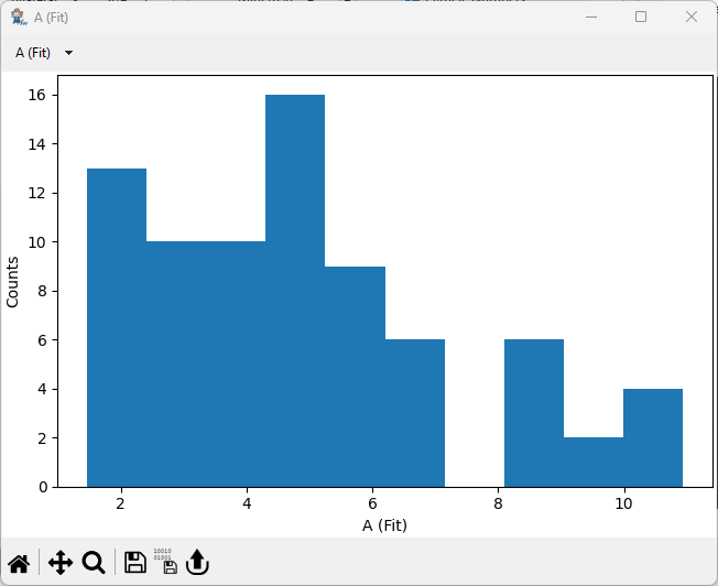
Fig. 8.13 The Parameter Distributions Window.#
Note
Parameter Distributions will automatically update when preprocessing or particle detection parameters are changed.
8.3. Image Statistics#
The Image Statistics window displays aggregate statistics of the entire image selected for analysis or, optionally, of a selected sub-region.
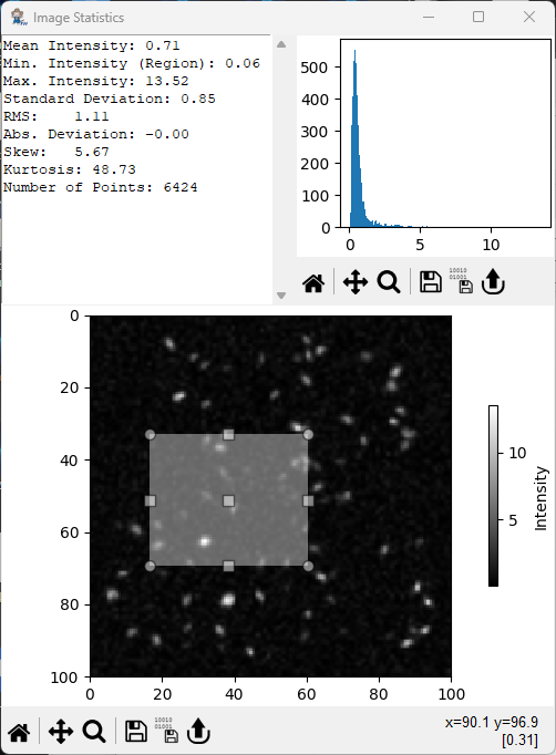
Fig. 8.14 The Image Statistics Window#
Parameters are:
Mean Intensity: The mean intensity of the image / region (8.2).
(8.2)#\[ \overline{x} = \frac{1}{N}\sum_{i=1}^N { x_i} \]Min. Intensity: The minimum intensity in the image / region.
Max. Intensity: The maximum intensity in the image / region.
Standard Deviation: The standard deviation of the intensity in the image / region (8.3).
(8.3)#\[ \sigma = \sqrt{\frac{1}{N-1}\sum_{i=1}^N{\left( x_i - \overline{x}\right)^2}} \]RMS: The root mean square deviation in the image / region (8.4).
(8.4)#\[ \chi = \sqrt{\frac{1}{N}\sum_{i=1}^N{ x_i^2}} \]Absolute Deviation: The absolute deviation in the image / region (8.5).
(8.5)#\[ AD = \frac{1}{N}\sum_{i=1}^N \lvert x_i - \overline{x}\rvert \]Skew: The skewness of the intensity distribution of the image / region (8.6).
(8.6)#\[ skew = \frac{1}{N}\sum_{i=1}^N \left( \frac{ x_i - \overline{x}} {\sigma}\right)^3 \]Kurtosis: The kurtosis of the intensity distribution of the image / region (8.7).
(8.7)#\[ kurt = \left[ \frac{1}{N}\sum_{i=1}^N \left( \frac{ x_i - \overline{x}} {\sigma}\right)^4 \right] -3 \]Variation: The coefficient of variation of the image / region (8.8).
(8.8)#\[ CV = \frac{\sigma}{\overline{x}} \]Number of Points: The number of points \(N\) in the image / region.
The underlying intensity distribution is displayed in the top right corner of the window.
Subregions of the image can be selected by dragging in the image plot (see The Image Statistics Window for an example).
8.4. Practical Considerations#
This section contains tips and tricks for successful particle analysis.
when analyzing images originating from spectral mappings, where the total number of points is commonly quite low, upsampling the image can aid both particle detection and fitting.
particle detection by thresholding relies on a global threshold which separates background and signal. If the image background is non-uniform, global thresholding will either result in
missing particles
the identification of background regions as ‘particle’.
Background removal can reduce or even entirely eliminate background uneveness to allow successful particle segmentation by thresholding.
Spurious noise can be eliminated by filtering. Alternatively, upsampling can also reduce the (relative) effect of noise.
For particles with meaningful shapes, e.g. cylindrical particles, use thresholding. For speckle images, where particles appear as small, circular blob, use local maximum detection.
fitting works best with large bounding boxes and approximately elliptical particles. More datapoints will greatly help the fit converge.
thresholding can merge several adjacent particles of similar intensity into a single blob. To alleviate this, segmentation can be used to separate the merged particles. Successful segmentation can be assessed in the bottom image of the thresholding pane where particles are indicated by different colors.
the Relative Height parameter of local maximum particle detection is a fraction of the maximum intensity and should be adjusted if the overall intensity of the image changes, e.g. after background subtraction.
Particle Analysis is can provide relevant information even for mappings that don’t contain discrete “particles”, i.e. the area occupied by specific chemical entities.
Emulsion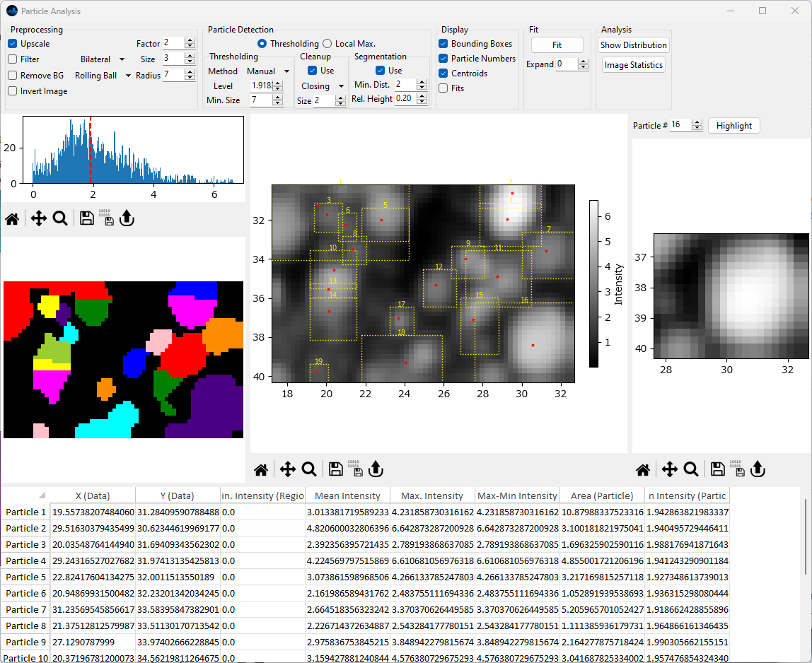 Area
Area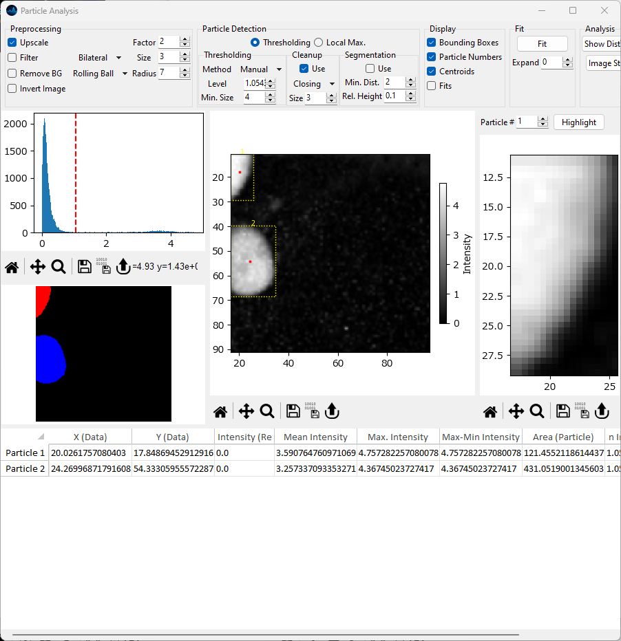
Fig. 8.15 Chemical entities area analysis#