6. Automated Image Formation

This section describes how to use automated, unsupervised processing to extract pure spectral components and their distributions from a dataset containing many spectra. SMDExplorer provides four different techniques to accomplish this:

• non-negative matrix factorization NMF

• principal component analysis PCA

• multivariate curve resolution MCR

• K-Means clustering

The section General Introduction will provide a theoretical background, the sections on the individual techniques will discuss the merits and shortcomings of each method, the section Automated Image Formation - A How-to will provide a hands-on tutorial on how to apply Automated Image Formation on a real-world dataset, and the section Display Options discusses the visualization options available in SMDExplorer.

Note

While this section is titled Automated Image Formation, the decomposition techniques outline here are applicable to one- or three-dimensional data as well.

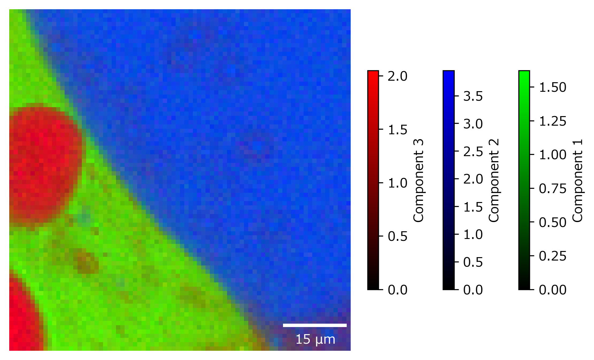
Fig. 6.1 Chemical component mapping using Automated Image Formation.

6.1. General Introduction

While three techniques (NMF, PCA, MCR) differ in the underlying mathematical approach, applicable data, and ultimate outcome, they all share the common idea of dimensionality reduction. Here, dimensionality is the product of number of spectra \(m\) and number of spectral channels \(n\). Dimensionality reduction techniques attempt to approximate the original dataset \(X\), which can be visualized as an \(n \times m\) matrix, by the product of two much smaller matrices \(W\) and \(H\), which have the dimensionality \(k \times m\) and \(n \times k\), respectively, with \(k \ll min(m,n)\) (see Dimensionality Reduction). In this example, the matrix \(W\) would contain the concentration (amount) of each component \(k\) as function of \(m\) (for example time) whereas the matrix \(H\) contains the pure spectral components \(k\). In contrast, K-Means clustering relies on grouping spectra by similarity, which will be discussed separately.

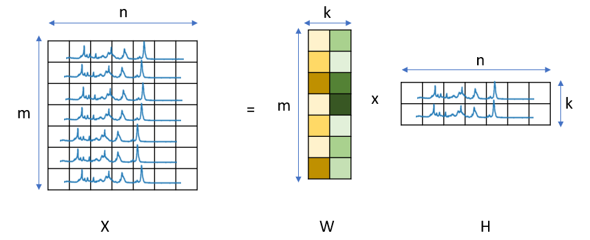
Fig. 6.2 Dimensionality Reduction

We can explore this problem on a toy dataset with a known answer.

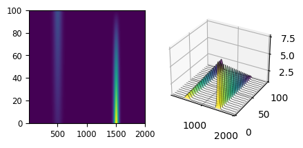
Fig. 6.3 A Toy Dataset

The dataset in A Toy Dataset shows two peaks (centered at 500 and 1500) that show intensity changes while spectra are recorded: In spectrum 0, the peak at 1500 has high intensity whereas in spectrum 100, the peak at 1500 has mostly disappeared while the peak at 500 has increased in intensity. This kind of profile might result from a chemical reaction that is monitored as time progresses. The goal of Automated Image Formation is to extract the pure spectral profiles as well as their distribution from this dataset. The solution to this toy problem is shown in A Toy Dataset - Components & Distribution.

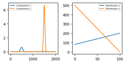
Fig. 6.4 A Toy Dataset - Components & Distribution

6.2. Non-negative Matrix Factorization

Non-negative Matrix Factorization (NMF) attempts to find two non-negative matrixes \(W\) and \(H\) to approximate the non-negative matrix \(X\). This implies that the spectra in \(X\) at each row \(m\) is the sum of the pure spectral components in \(H\) weighted by their concentrations in \(W\). This results in pure spectral components that are readily interpretable, as illustrated in the solution to our to problem. While the order of the components is reversed, the decomposition procedure was able to separate the two different components and extract their distributions.

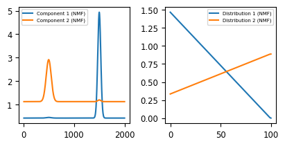
Fig. 6.5 The Toy Dataset - NMF Decomposition

In SMDExplorer, automated image formation by NMF is available in the Decomposition pane by selecting NMF from the Method drop-down menu (see Automated Image Formation - NMF Decomposition).

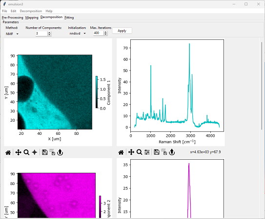
Fig. 6.6 Automated Image Formation - NMF Decomposition

Parameters

Number of Components

The number of different components in the dataset (\(k\) in Dimensionality Reduction).

Initialization

The initial guesses for the matrices \(W\) and \(H\).

• nndsvd: Non-negative double single value decomposition (Boutsidis, 2008). This is a good choice if sparseness (non-overlapping components) is desired.

• nndsvda: Non-negative double single value decomposition with zero values filled by the average of \(X\). This is a good choice if sparseness is not required.

• random: Initialization with random values.

Max. Iterations

The maximum number of iterations to perform when optimizing the solution for \(X = W \times H\). SMDExplorer will display a warning if the maximum number of iterations has been reached before convergence.

For many spectral datasets, especially in Raman spectroscopy, the assumption non-negativity constraint of NMF and the assumption that spectral mixtures are simply the weighted sum of the pure components is justified. This makes NMF a well-suited method for automated image formation since the resulting pure components strongly resemble actual spectra. As a result, interpreting NMF results is straightforward.

Note

Non-negativity is enforced by subtracting the minimum value from the dataset - regardless whether negative values are present or not.

6.3. Principal Component Analysis

PCA attempts to project the original dataset \(X\) into a lower-dimensional space while retaining as much of the original variance as possible. This is achieved by identifying the principal components, which are orthogonal vectors that capture the maximum variability of the data. These components form the new axes of the transformed space, with the first principal component capturing the most significant variation, followed by the second, and so on. While this property makes PCA an excellent choice for extracting a sparse representation of the dataset (see Statistical Denoising), the pure components extracted by PCA are often difficult to interpret. As there is no assumption of non-negativity (unlike NMF), negative spectral intensities or distributions often yield mathematically correct but non-physical solutions. This becomes apparent in The Toy Dataset - PCA Decomposition.

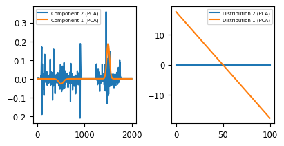
Fig. 6.7 The Toy Dataset - PCA Decomposition

The PCA algorithm extracts one meaningful principal component (orange), with a a concentration profile that includes positive and negative regions and a pure spectrum that contains a positive and negative peak. The second extracted component (blue) contains purely noise and is constant throughout the dataset. While this solution is mathematically correct (it solves the equation \(X = W \times H\)), the result of NMF clearly is easier to interpret and arguably more meaningful.

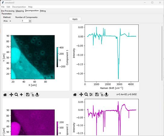
Fig. 6.8 Automated Image Formation - PCA Decomposition

This shortcoming also becomes apparent when performing PCA decomposition on a real-world dataset. For typical datasets, NMF or MCR will result in more meaningful pure spectral components and distributions.
In SMDExplorer, automated image formation by PCA is available in the Decomposition pane by selecting PCA from the Method drop-down menu.

Parameters

Number of Components

The number of different components in the dataset (\(k\) in Dimensionality Reduction).

Note

In contrast to many PCA implementations, SMDExplorer only centers the data but performs no additional scaling (“Whitening”) by default. If Whitening is desired, this can be activated using the Whitening option. The Poisson whitening method implements the noise-corrected PCA method introduced by Le Marois et al..

6.4. Multivariate Curve Resolution

Similar to NMF, Multivariate Curve Resolution (MCR) attempts to disentangle and quantify individual components of mixtures of overlapping signals. While the two techniques originate from different fields, their algorithms share many similarities and tend to produce closely matched results. Most importantly, MCR shares the non-negativity assumption with NMF, which gives rise to meaningful spectra and concentration curves. This becomes immediately evident when applying MCR decomposition to the the toy dataset.

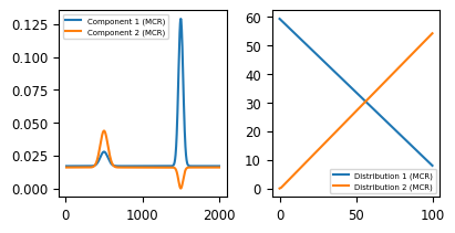
Fig. 6.9 The Toy Dataset - MCR Decomposition

In SMDExplorer, automated image formation by MCR is available in the Decomposition pane by selecting MCR from the Method drop-down menu (see Automated Image Formation - MCR Decomposition).

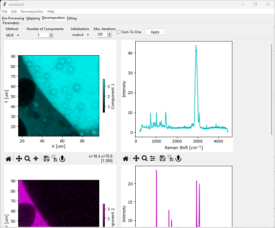
Fig. 6.10 Automated Image Formation - MCR Decomposition

Parameters

Number of Components

The number of different components in the dataset (\(k\) in Dimensionality Reduction).

Initialization

The initial guesses for the matrices \(W\) and \(H\).

• nndsvd: Non-negative double single value decomposition (Boutsidis, 2008). This is a good choice if sparseness (non-overlapping components) is desired.

• nndsvda: Non-negative double single value decomposition with zero values filled by the average of \(X\). This is a good choice if sparseness is not required.

• svdabs: Initialization with the absolute value of the single-value decomposition.

• NMF: Initialization with the results of an NMF decomposition

Max. Iterations

The maximum number of iterations to perform when optimizing the solution for \(X = W \times H\). SMDExplorer will display a warning if the maximum number of iterations has been reached before convergence.

Sum-to-one

Requires that the relative concentrations at each location equal 100%, i.e. there are no components unaccounted for.

The choice between NMF and MCR does, for many datasets, come down to personal choice and preference and the results of the two algorithms are, for well-behaved datasets, often quite comparable, especially in the absence of a ground truth solutions that is known a priori. The high interpretability of both the spectra of the pure components as well as their concentration profiles makes both NMF and MCR better choices than PCA.

6.5. K-Means Clustering

K-Means clustering partitions the sample spectra into \(k\) clusters, with each spectrum belonging to the nearest cluster center. This is achieved by minimizing inter-cluster distances, which, in our case, is the Euclidian distance between spectra.

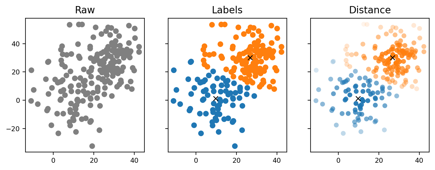
Fig. 6.11 K-Means Clustering

Each spectrum is assigned a label that indicates the cluster it belongs to. When using these labels for image formation, the resulting images take a binary, comic book-like appearance. Alternatively, one can use the distance from the cluster center for image formation. This metric describes the similarity of each spectrum to the prototypical cluster center.

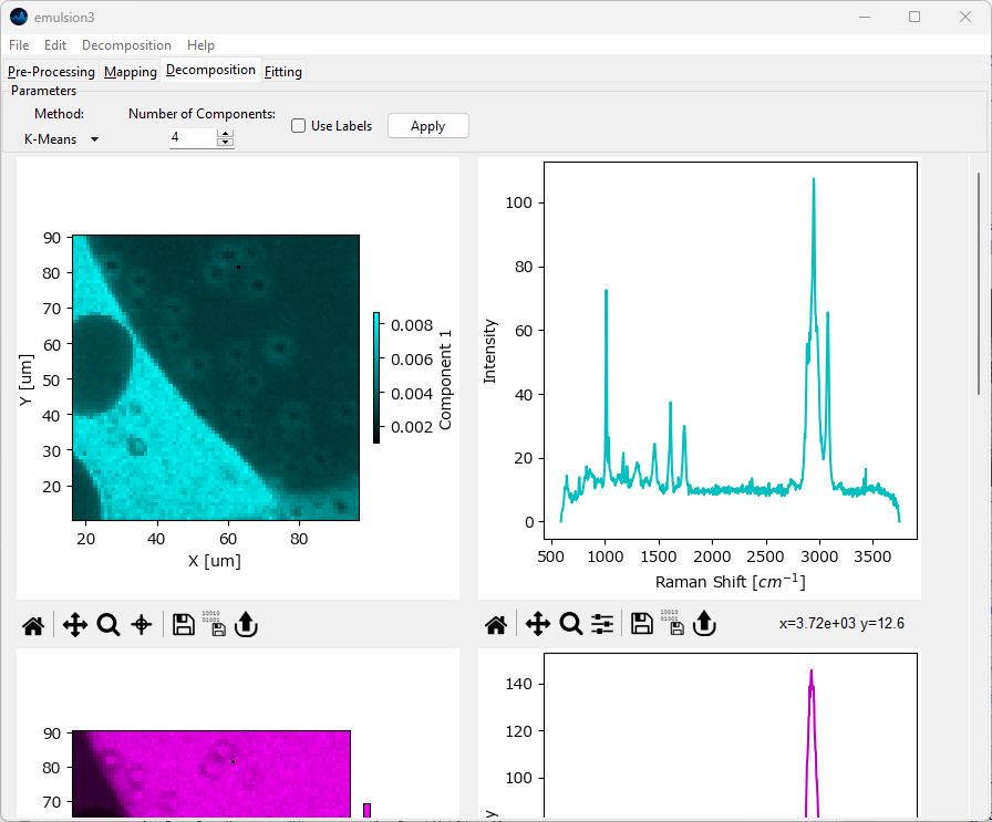
Fig. 6.12 Automated Image Formation - K-Means Clustering

Parameters

Number of Components

The number of clusters to partition the data into

Use Labels

When checked, use the assigned cluster labels to form images / profiles. This will result in binary (on/off) images. When unchecked, the distance from the cluster center is used instead.

The spectra displayed in the right column are:

• the arithmetic mean of all spectra belonging to a cluster weighted by the inverse of the distance from the cluster center if Use Labels is unchecked

• the arithmetic mean of all spectra belonging to a cluster if Use Labels is checked.

Note

K-Means clustering is highly dependent on initialization conditions (the starting guesses for the centers of the clusters). This means that the algorithm won’t neccessarily converge to the same solution for every run.

Distance

Label

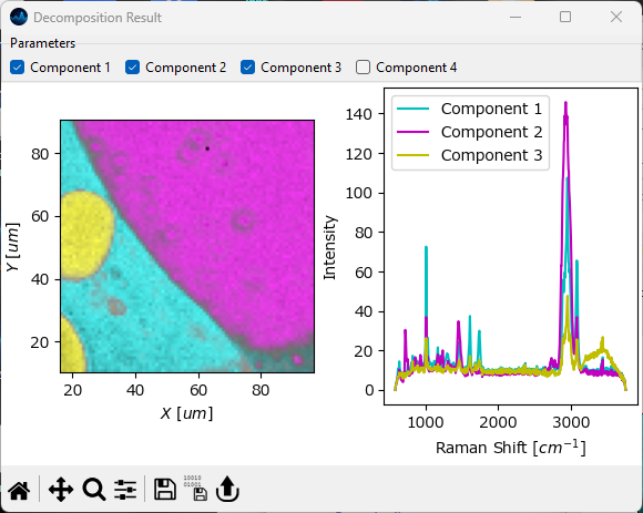
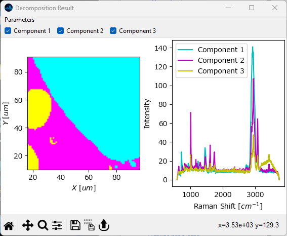
Fig. 6.13 K-Means Clustering - Distance vs Label

Note

When K-Means clustering is performed with Use Labels turned on, the spectra assigned to each cluster can be exported individually using Decomposition ‣ Export Cluster and selecting the desired cluster number. Please note that the exported spectral series / spectral database contains the spectra only (in the order they were recorded); all temporal / spatial information is lost as clusters are not neccessarily continuous. This feature can be used to split a dataset, for example a time scan, into different categories based on spectral similarity, for example to remove blinking in surface-enhanced Raman spectroscopy (SERS) experiments.

6.6. Automated Image Formation - A How-to

This section outlines how to perform Automated Image Formation on a real-world dataset.

Important

While Automated Image Formation provides a convenient and quick way to extract pure spectra and concentration profiles from datasets, care must be taken not to overinterpret the results. There are many mathematically equally valid solution to the decomposition problem and while both NMF and MCR do a good job of providing generally sensible solutions, the decomposition result should be considered as a (good) starting point for further manual investigation rather than the final outcome.

Two factors are key to obtaining meaningful decomposition results:

• suitable data preprocessing

• appropriate choice of the number of components

Suitable pre-processing steps typically include:

1. selecting the relevant spectral range, i.e. removing parts of the spectra that contain no meaningful data. This can be achieved by Range Selection.

2. Removal of cosmic ray artifacts (if present). High intensity cosmic ray spikes, especially if abundant, can mislead the decomposition algorithms and mask meaningful spectral features. This can be achieved by Cosmic Ray Removal (Despiking).

3. Baseline subtraction. Unlike PCA, which operates on mean-subtracted data, NMF and MCR performs the decomposition on the original dataset. This means that the absolute intensity (including the baseline) is taken into account during decomposition. Setting the baseline to small values close to zero effectively results in emphasizing the larger, positive data and less weight being assigned to the baseline. Baseline subtraction can be achieved by either the Simple Baseline Removal (Bring to Zero) or the Non-linear Baseline Removal functions in the Preprocessing Window.

4. Normalization (if required and meaningful). If the intensity within a spectral range (or across the entire spectrum) of the dataset is expected to be constant throughout the experiment, normalization can be performed, for example to counter the effect of focal drift.

Note

To ensure non-negativity, the minimum value of the data is subtracted from the dataset prior to decomposition. This can, in some cases, serve as an alternative to baseline subtraction during preprocessing. Manual baseline subtraction is, however, still recommended for best decomposition results.

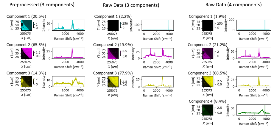
Fig. 6.14 Automated Image Formation Hands-On - Preprocessing

The figure Automated Image Formation Hands-On - Preprocessing contains the Automated Image Formation result by NMF using raw (center and right columns) and preprocessed data (left column). While the result using raw data (center) is certainly workable, high-intensity cosmic ray artifacts lead to the mis-assignment of one component. This can be alleviated by adding an additional component (right column).

The example in Automated Image Formation Hands-On - Preprocessing also illustrates the importance of selecting the appropriate number of components. Ideally, the number of spectrally different entities in the sample is known ahead of time and can inform this choice. Otherwise, the number of components has to be optimized manually. The following heuristics may be useful:

• An explained variance plot (computed via PCA) can be accessed via Decomposition ‣ Explained Variance. Inflection points in this plot can provide good starting values for the number of components parameter. In Automated Image Formation Hands-On - Explained Variance, the explained variance (blue) has a plateau up to five components and then drops significantly. Hence five components might be a good starting value. In this particular dataset, the optimum number of components for raw data turns out to be four, which is due to the different treatment and weighting of high-intensity cosmic rays by PCA and NMF.

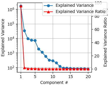
Fig. 6.15 Automated Image Formation Hands-On - Explained Variance

• If the number of components is too high, two components will share the same (or a very similar) spectral signature and a similar concentration profile / spatial distribution.

• If the number of components is too low, there will typically be a convergence warning by the NMF or MCR algorithm since the original dataset cannot be properly reconstructed from the decomposition result.

Note

The algorithms in Automated Image Formation are generally not very sensitive to noise in the dataset, especially when the number of spectra is high. Consequently, smoothing or denoising are typically not required and can, in the case of statistical denoising, even be detrimental as the sparse output of statistical denoising removes information from the dataset.

6.6.1. Whitening

Whitening refers to (reversible) scaling the data according to statistical assumptions. Scaling the data before decomposition can help the decomposition algorithm converge, especially when spectra or spectral channels vary strongly. SMDExplorer offers two whitening methods:

• scaling by the standard deviation. This implies that channels / features follow a normal distribution and is most appropriate for Raman data. This option is available in the Whitening option menu as Gauss for NMF, PCA, MCR, and K- Means.

• scaling by the square root of the mean. This implies Poissonian noise and is most suitable for photon counting data. This option is available in the Whitening option menu as Poisson for NMF, PCA, MCR, and K-Means.

See also

The Poisson option implements the whitening procedure outlined in Masia et al. for the unsupervised analysis of fluorescence lifetime imaging data.

The Poisson whitening option for PCA analysis implements the noise-corrected PCA (NC-PCA) procedure introduced in Le Marois et al.

Note

For PCA, whitening only scales the intensities (channels) while both samples (sampling locations) and channels are (reversibly) scaled in the other methods. This follows the algorithms outlined in the papers cited above.

6.7. Display Options

SMDExplorer includes several options to visualize images / intensity profiles obtained from the dimensionality reduction methods available in the Decomposition window.

1. The first option is the results the Decomposition window itself. After selecting a Method, Number of Components, and Initialization, and clicking Apply, the Decomposition result will be displayed in the pane below.

   • the left column contains the concentration profiles / spatial distribution of each component

   • the right column contains the spectrum of the pure component

   Each graph can be interacted with individually, for example by zooming, panning, or changing the color scale. The data contained in each graph can be exported and graphs can be saved as individual images, just like any graph in SMDExplorer.

   Note

   Depending on the number of components selected for Automated Image Formation, you may have to scroll down to see the entire result.

   

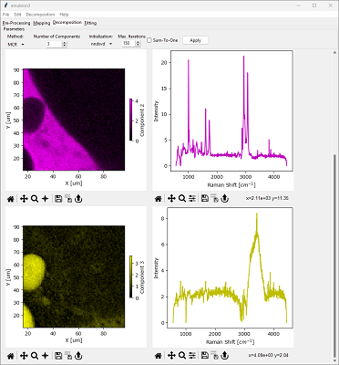
   Fig. 6.16 Automated Image Formation - The Decompositon Window

   By default, SMDExplorer uses a different color for each component in the Decomposition window. This can be turned on or off using the Decomposition ‣ Cycle Colors menu item or by manually assigning a different color scheme to a graph.

2. The Decomposition Result window, available via the Decomposition ‣ Export Figures menu item. This window contains the outcome of the Automated Image Formation procedure in a single figure. In addition, the concentration profiles also contain the relative abundance of each component (calculated assuming that the total concentrations at each location sum to unity).

   Hint

   Adjust the size and aspect ratio of the Decomposition Result window to yield a visually pleasing figure.

   

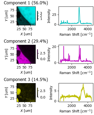
   Fig. 6.17 Automated Image Formation - The Decompositon Result Window

3. The Overlay Window. In this window, concentration profiles / distributions and pure spectral components are displayed in a single graph, with the different components indicated by different colors and their relative abundance indicated by the color intensity. Individual components can be enabled or disabled for display by the row of checkboxes at the top of the window, similar to Comparing Intensity Profiles / Images.

   

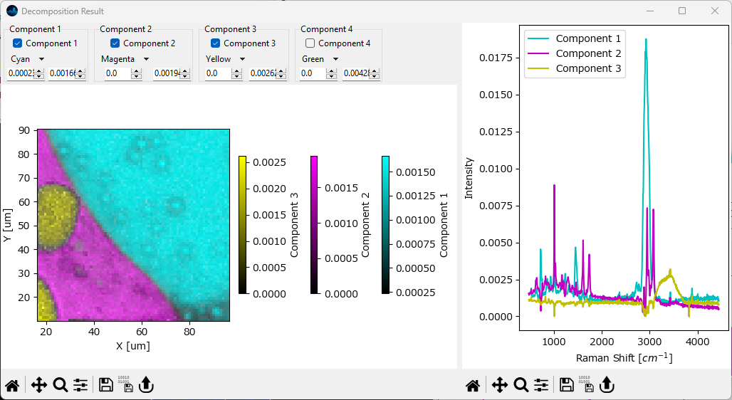
   Fig. 6.18 Automated Image Formation - The Decompositon Overlay Window