3. General Usage#
The section contains instructions and remarks on how to make best use of SMDExplorer. For details on data preprocessing, manual or automated data visualization, and peak deconvolution, please see the relevant sections.
3.1. File Input / Output#
3.1.1. Input#
SMDExplorer can read and process the following file types:
.smdfiles originating from the TII Nanofinder software. These files typically contain spectral mappings or kinetic scans acquired with one or more spectral detectors. When more than one detector channel is present in the file, for example when the dataset contains both Raman and Brillouin spectra acquired simultaneously, SMDExplorer will display a prompt to let you decide what type of spectra to import. The section Analysis of Spectral Mappings contains further information how to process this data.
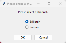
Fig. 3.1 The Channel Prompt#
Hint
To compare different channels of the same dataset, different datasets, or the same dataset processed differently, simply open the same file repeatedly in SMDExplorer.
.s1dfiles originating from the TII Nanofinder software. These files typically contain a single spectrum or a kinetic series, i.e. an time interval scan of spectra. SMDExplorer permits opening multiple.s1dfiles containing single spectra in a single window at the same time for easy comparison and processing. The section Analysis of Individual Spectra contains further information how to analyze and process individual spectra. If the.s1dfile contains a time series, only one file can be open in a single window at a time. Please see the section Analysis of Spectral Mappings for further details..mdtspectral databases originating from the TII Nanofinder software containing a number of different, independent spectra. SMDExplorer permits opening multiple.mdtin a single window for comparison. The section Analysis of Individual Spectra contains further information how to analyze and process individual spectra..hdf5files containing multi-point Raman mappings originating from the TII Phalanx instrument and the Igor Pro software controlling this instrument. Please see the section Igor Pro HDF5 export for details on Igor Pro interoperability..hdf5files originating from SMDExplorer that contain exported raw or preprocessed data that consists of either a number of individual spectra or spectral mappings.
Hint
For spectroscopic data (Raman, Brillouin, Fluorescence, etc.), the type of spectrum can be changed via .
3.1.2. Output#
Interoperability is a primary objective of SMDExplorer. To this end, data can be converted to a number of different output formats for processing in third-party software as well as re-imported into SMDExplorer for further analysis (roundtripping).
        flowchart TD
    A((.smd scan)) --> B((.hdf5 scan))
    A -.-> C{{.mat Matlab file}}
    %% A --> |preprocessed data| A
    A -.-> G
    A & B -.-> |single spectra| F
    B --> |interoperability| A

    E[.s1d kinetic series] -.-> A
    E-.-> B
    E -.-> C
    E-.-> G

    G((.mdt)) -.-> |multi-spectra| A
    G <-.-> F([.hdf5 multispectrum])
    G-.->C
    %% G-.->G
    H[.s1d single spectrum] -.-> F
    H-.->C
    H-.->A
    H-.->G

    J{{.csv}}
    G-.->J
    H-.->J
    A-.-> |single spectra| J
    B-.-> |single spectra| J

    K{{JCAMP-DX .jdx}}
    G-.->K
    H-.->K
    A-.-> |single spectra| K
    B-.-> |single spectra| K
Fig. 3.2 File Input / Output / Conversion by SMDExplorer. Input-only formats are shown as rectangles, output-only formats as diamonds, input-output formats as circles / rounded rectangles.#
spectral mappings (
.smd) can be converted to and from the.hdf5format with full roundtripping support. This allows taking advantage of the different analysis and processing features of SMDExplorer, TII Nanofinder, and third-party software capable of reading.hdf5files.individual spectra (
.mdtor several.s1d) can be converted to.hdf5spectral databases (.hdf5multi-spectrum).sets of individual spectra (
.mdtor.s1d) can be converted to an.smdscan.spectra of interest from an
.smdscan can be converted to an.mdtdatabase.data can be exported as
.matMatlab files.Note
Since Matlab also provides
.hdf5support, this format is preferred to the native.matformat due to richer meta-data support and the possibility of roundtripping.the data contained in graphs can be directly exported in the
.csvor JCAMP-DX (.jdx) format, either as a file or to the clipboard. Please see the the section on Graphing for details. In addition, traces can be exported as a multi-spectrum.hdf5file or an.mdtdatabase.
3.2. Acquisition Parameters#
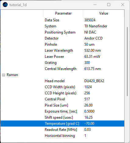
Fig. 3.3 The Acquisition Parameters Window.#
Acquisition parameters of spatial or temporal scans are available via . Acquisition parameters include:
detector properties, e.g. exposure times, number of accumulations, readout mode, etc.
spectrometer properties, such as the grating size of the pinhole used
stage properties, e.g. extent and resolution of the scan axes
general file properties
Note
Please note that the number of persisted acquisition parameters varies between file formats.
Parameters can be selected and copied to the system clipboard.
3.3. Graphing#
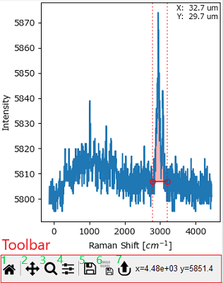
Fig. 3.4 An SMDExplorer Graph#
Graphs are the main user interface component of SMDExplorer to interact with and analyze data. While the layout and controls of some graphs will change depending on their content, all graphs have some aspects of navigation and user interaction in common.
The Toolbar at the bottom of each graph gives access to zooming and resizing controls and allows exporting the data displayed in the graph.
Interactive Controls in the graph window allow the manipulation of certain parameters of processing or analysis interactively. For example, the dashed red vertical lines in the example graph allow selecting a spectral range for computation of running sum of the spectral intensity.
Note
The cursor will change when hovering over an interactive Control.
Interactive Controls cannot be manipulated when the graph is in pan or zoom mode.
The Toolbar contains the following elements (from left to right in Figure 3.4):
The Autoscale button. This will rescale all axes (and color scales, if applicable) to match the limits of the dataset. Autoscaling can also be achieved with the keyboard shortcut Ctrl-A (⌘-A on macOS).
The Pan button. Clicking this button activates the pan mode, clicking the Pan button again restores normal graph navigation. In pan mode, you can change the range of the displayed data when dragging in the graph window while holding down the left mouse button. Holding down the right mouse button while dragging will zoom in or out of the graph. Pan mode can also be activated by holding down the Alt key.
The Zoom button. Just like the Pan button, the Zoom button activates or deactivates the zoom mode. In zoom mode, you can select a rectangular area of the graph to magnify while clicking and dragging in the graph while holding down the left mouse button. Clicking and dragging while holding down the right mouse button will demagnify (unzoom) the selected area.
Zoom mode can also be activated by holding down the z key.
Hint
Holding down the x key will restrict panning or zooming to the horizontal axis, holding down the y key will restrict panning or zooming to the vertical axis. Panning and Zooming work on color scales as well.
The Configure button. This button will display options to customize data display or autoscaling:
Autoscale Visible: When active, the range of the vertical axis will be adjusted to match minimum and maximum of the visible horizontal selection of the currently displayed trace or spectrum. This requires having selected a horizontal x-range by zooming or panning while holding down the x key.
Show Grid: Displays a grid.
Note
The Configure button is only available for one-dimensional graphs.
The Save button. This will save the graph to disk in various file formats.
The Save Data button. This will save the data displayed in the graph to disk as a
.csv,.hdf5, JCAMP-DX.jdx, or.mdtdatabase file allowing further analysis in third-party software. For two-dimensional data,.hdf5and.tiffexport are also available.
The Copy Data button. This will copy the data displayed in the graph to the system clipboard.
Important
Keyboard shortcuts in graphs only work if a graph is active. The active graph is indicated by a black outline. To activate a graph, simply click anywhere on the graph using the mouse.
Hint
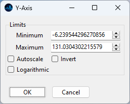
Fig. 3.5 The Axis Dialog#
For more fine-grained control, the axis (or color scale) limits can also be set by double-clicking on an axis and entering the lower or upper limit in the axis dialog window.
- Autoscale
Selecting autoscale will autoscale the selected axis (unlike the Autoscale button that will autoscale all axes).
- Invert
Inverts the axis or colorscale
- Logarithmic
Switches between logarithmic and linear and scaling of the selected axis.
Additional display options are available for plots containing two- and three-dimensional data. Please also see the remarks on tweaking 2D and 3D graphs when plotting multidimensional data.
Hint
Axis limits can also be adjusted using the mouse scroll wheel or trackpad scrolling events. To zoom into our out of a graph, first activate it by clicking on the graph. Next, move the scroll wheel or two-finger drag on the touchpad to zoom while the cursor is placed within the axes of the graph. As discussed above, holding down the x key will restrict zooming to the horizontal axis, holding down the y key will restrict zooming to the vertical axis.
Hint
Graphs can be exported to the system clipboard using default system keyboard shortcuts.
3.4. Analysis of Individual Spectra#
SMDExplorer allows the processing, analysis, and comparison of multiple individual spectra contained in an .mdt or multiple .s1d files (see Input).
Hint
Additional files can be appeneded to the currently selected list of spectra by .
The list of loaded spectra is displayed in the Spectra sidebar on the left. The right pane of the SMDExplorer contains different analysis panes:
the Browse pane allows the display and comparison of multiple spectra.
the Preprocessing pane allows applying processing steps , e.g. background subtraction or smoothing, to the selected spectrum.
the Fitting pane allows performing peak deconvolution using curve fitting to determine peak positions / peak widths of the selected spectrum.
You can switch between the panes by clicking on the tab title at the top, by the Control-Tab (for forward switching) or Ctrl-Shift-Tab (for backward switching) keyboard shortcuts, or by using the Alt-firstLetter where firstLetter is the first, underlined letter of the tab title (e.g. Alt-F for the Fitting pane).
See also
Please see the sections on Preprocessing and Peak Deconvolution for details on data processing and peak deconvolution.
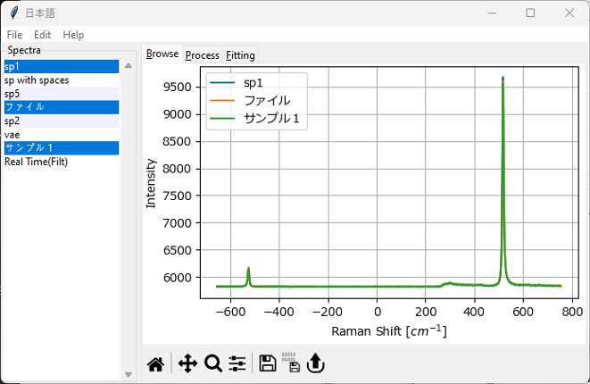
Fig. 3.6 The Browse Window#
Tip
In the Spectra sidebar, multiple spectra can be selected by clicking while holding down the Ctrl or Shift keys. All spectra can be selected using the shortcut Ctrl-A.
A context menu can be accessed by right clicking on the Spectra sidebar. This menu gives access to the following functions:
Delete - deletes the spectrum from the display list in the Spectra sidebar.
Rename - allows choosing a new name for the spectrum.
Change Spectrum Type - allows changing the spectral axis (x axis) from Raman Shift [cm-1] to Brillouin Shift [GHz] and vice versa.
Modify Trace - allows scaling / offsetting the trace and selecting the trace color (Figure 3.7)
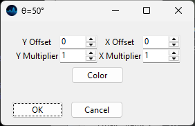
Fig. 3.7 The Modify Trace Dialogue#
Match Height scales spectra between 0 and 1 for easy inspection. For more control over scaling, use the Normalization preprocessing step.
Tip
The Delete and Change Spectrum Type functions can be applied to multiple spectra at once.
Export as Series - allows export of the selected spectra as an
.hdf5or.smdspectral scan. The scaling of the spectral series can be adjusted using the Series Export Dialogue.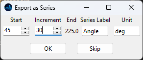
Fig. 3.8 The Series Export Dialogue#
Parameters
- Start
The first value of the series
- Increment
The increment between the measured spectra
- Series Label
The label to be applied to the series - this will be displayed on the horizontal axis.
- Unit
The unit of the measured data
Note
Series export will be performed in the order of selection in the Spectra sidebar.
Stitch performs spectral stitching of spectra acquired at overlapping wavelength ranges (Figure 3.9).
Note
Spectral stitching is performed in order of selection in the Spectra sidebar. This menu item is only available if
all spectra are of the same type
consecutive spectra have an overlapping spectral range
Stitching is performed by the following algorithm:
Identify the overlappingspectral region
Note
The spectral coordinate is expected to increase between consecutive spectra.
Use interpolation to find the intensity values of the second spectrum that correspond to the spectral coordinates of the first spectrum in the overlap region.
Note
Spectral coordinates in the overlap region are taken from the first spectrum of the spectral pair. Calibration can be used to compensate for offsets in the spectral coordinate between spectra, for example offsets due to play or backlash in the positioning mechanism of the grating of the spectrometer. A convenient way to do this is to overlay two adjacent spectra and check for coincidence of spectral features in the overlap region.
Linearly interpolate between the intensity values of the first and second spectrum in the overlap region.
Note
Linear interpolation between the two adjacent spectra avoids sharp offsets between spectra as long as spectral intensities are roughly constant. If the baseline changes significantly between spectra (for example due to bleaching of a fluorescent background), background subtraction or non-linear baseline removal can be used to pre-process spectra prior to stitching.
Append the intensity values of the second spectrum outside the spectral region of the second spectrum to the stitched spectrum
Repeat for the next spectrum.
Overlapping spectra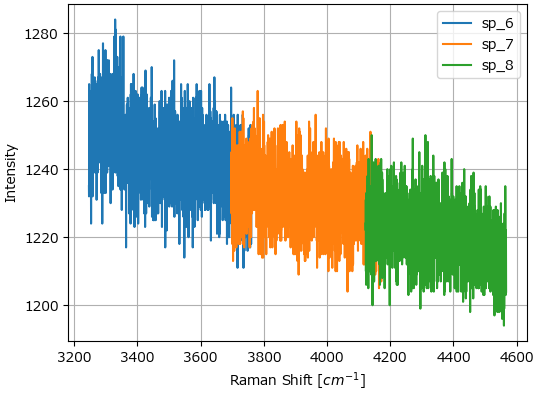 Stitched spectrum (red)
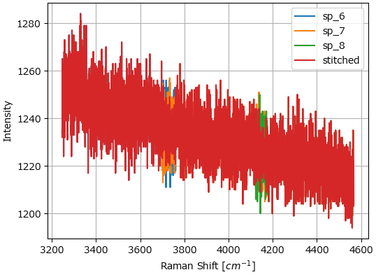
Fig. 3.9 Spectral Stitching#
3.5. Analysis of Spectral Mappings#
Spectral mappings consist of multiple related spectra obtained from the same sample at defined spatial positions or during a time interval scan. A mapping dataset can be opened from an .smd or .s1d (for interval scans) file for data originating from Nanofinder instruments or from a .hdf5 file for data originating from a Phalanx instrument. In addition, SMDExplorer can also be used to convert between these formats and to save preprocessed data.
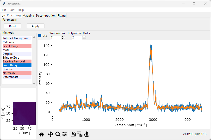
Fig. 3.10 Analysis of Spectral Mappings#
SMDExplorer offers the following functions for processing and analysis of spectral mappings:
Preprocessing gives access to a variety of preprocessing techniques, e.g. smoothing, denoising, cosmic ray artifact removal, or baseline removal.
Mapping allows the analysis of spectral datasets by analyzing different spectral parameters, for example integrated spectral intensity across a given wavenumber range, and plotting this parameter against the spatial position.
Decomposition gives access to automated image formation methods. Rather than manually selecting a spectral parameter, Decomposition uses statistical techniques such NMF, PCA, or MCR to extract the relevant spectral components and their (spatial) distributions from the dataset in an automated fashion.
Fitting allows performing peak deconvolution by fitting spectra with different spectral line shapes, e.g. Lorentzians or Gaussians, to extract peak positions and peak widths. The peak deconvolution result can in turn be used to generate mappings or profiles.
The different analysis and processing options are available via the four tabs at the top of the SMDExplorer window. You can switch between the tabs using Ctrl-Tab (forward) and Ctrl-Shift-Tab (backward).
Important
Data preprocessing is typically the first step performed during analysis. The data displayed in the Mapping, Decomposition, and Fitting panes will contain the preprocessed data if you have selected and activated preprocessing steps and clicked Apply in the Preprocessing pane. To return to the original dataset, click the Reset button in the Preprocessing pane. To adjust data preprocessing , first click the Reset button, change preprocessing parameters, and click Apply again. The data in the subsequent analysis panes will update accordingly. For details, see the section Remarks on Processing Datasets.
3.6. Preferences#
The Preferences window allows customizing SMDExplorer.
on Windows or Linux, the Preferences window can be accessed via .
on macOS, the Preferences window can be accessed from the
Appmenu or using the shortcut ⌘-,.
3.6.1. General Preferences#
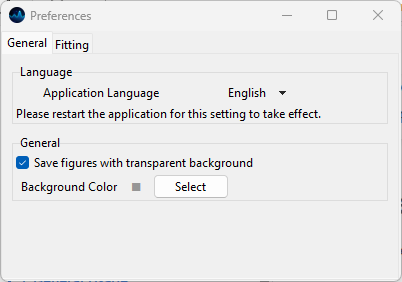
Fig. 3.11 General Preferences#
- Language
The General Preferences tab allows changing the application language. Currently, SMDExplorer is localized in:
English
German
Japanese
Please restart the app for the language change to take effect.
- Save figures with transparent background
If turned on, figures are saved with a transparent background. This allows embedding into slides with a non-white background color. When turned off, a white background and, for masked data, the selected background color, will be used instead.
- Background Color
Changes the background color of 2D or 3D graphs.
Note
This graph background is typically only visible if data has been masked. The default value is a light gray color to allow easy visualization of masked values.
3.6.2. Fitting Preferences#
The Curve Fitting Preferences tab allows changing settings for curve fitting (peak deconvolution):
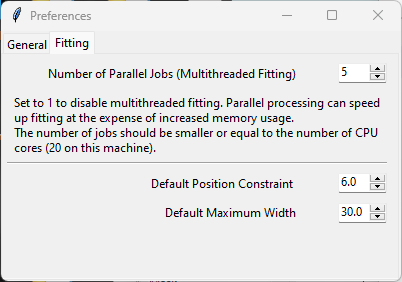
Fig. 3.12 Curve Fitting Preferences#
- Number of Parallel Jobs
How many curve fits should be performed in parallel when performing peak deconvolution on a large dataset. Since parallel execution (multithreading) has a non-insignificant overhead, peak deconvolution is only markedly sped up using parallel processing when number of peaks is > 1000. In addition, parallel processing also consumes significantly more memory, so increasing the number of parallel jobs can lead to system instability. The default (
4) provides a good compromise between speedup and memory consumption.
- Default Position Constraint
The permitted variation of peak position during peak deconvolution for newly added peaks. Increase the default value of
2.0to allow larger variations of peak position.- Default Maximum Width
The default width for newly added peaks during peak deconvolution. Adjust the default value of
30.0to match the peak shapes in your dataset.