4. Preprocessing

The section describes the data preprocessing techniques available in SMDExplorer.

4.1. Introduction

Data preprocessing is a key step prior to data analysis of spectral datasets. Preprocessing can help to enhance the desired signal, suppress unwanted spectral artifacts, and remove external experimental effects such as focus drift. SMDExplorer implements a number of preprocessing methods that can enhance the signal-to-noise ratio of the dataset to facilitate downstream analysis as well as data interpretation. This section gives an overview of the available techniques, the section Remarks on Processing Single Spectra provides details on how to process individual spectra, and the section Remarks on Processing Datasets describes how to process spectral datasets, for example interval of spatial scans.

See also

There is a large number of publications describing and benchmarking different preprocessing techniques, in particular denoising, smoothing, and baseline removal. For an overview, see Bocklitz, 2011.

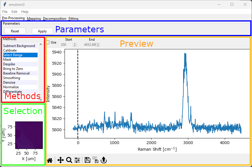
Fig. 4.1 The Preprocessing Window

The preprocessing window contains four areas:

1. the Parameters section with buttons to apply the currently configures preprocessing configuration to the data. The Reset button (for scans only) discards a previous preprocessing result and allows re-processing the data with a new parameter set.

2. The Methods section that allows switching between different preprocessing methods. Activated methods will be shown with a red background. Methods are applied to the dataset from top to bottom.

   Hint

   The order of preprocessing steps can be changed by dragging the items in the Methods list.

3. The Selection section (for scans only). This allows selecting which spectrum will be shown in the preview graph by clicking on the mapping / intensity profile.

4. The Preview section. This part of the window will update depending on the preprocessing method. Generally, the bottom of the Preview section contains a graph that shows a preview of the selected preprocessing steps. The top contains toolbar that allows adjusting various parameters of the preprocessing step. The checkbox Use at the top left activates or deactivates the preprocessing step.

4.1.1. Remarks on Processing Datasets

A typical preprocessing workflow for processing spectral datasets might be as follows:

1. (optional) adjust the spectral axis the data using the Calibration if required.

2. Crop the spectral range to a region of interest using Select Range.

3. (optional) remove cosmic ray artifacts using Despike if the dataset contains cosmic ray spikes.

4. remove the baseline using Baseline Subtraction

5. increase the signal-to-noise ratio of the dataset:

   • to smooth the spectra individually, use Smoothing

   • to denoise the dataset by averaging or truncated PCA, use Denoise

Note

In general, the default values of each of the preprocessing steps should provide a reasonable starting point that gives good results for most datasets. For a detailed discussion of the meaning and effect of each parameter, see the sections below.

Once you have adjusted the parameters of each of the steps above, click the Apply button in the Parameters pane to perform the preprocessing steps. You can analyze the processed data in the Intensity Profiles / Image Formation window. If you want to tweak your preprocessing pipeline, first click Reset to discard the previous preprocessing result, adjust parameters or add preprocessing steps, and click Apply again to re-process the data.

Hint

• preprocessed data can be saved to disk using File ‣ Save Preprocesed Data for analysis in third-party software or as a backup for further analysis in SMDExplorer.

Tip

• the currently selected preprocessing settings can be saved using Preprocessing ‣ Settings ‣ Save

• a saved set of preprocessing steps can be loaded from disk using Preprocessing ‣ Settings ‣ Load

• the currently selected preprocessing settings can be applied to other files using using Preprocessing ‣ Batch Process

Saved processing steps include:

• Background subtraction (including custom background data)

• calibration

• range selection

• cosmic ray removal

• simple and non-linear baseline removal

• smoothing

• denoising

• normalization

• differentiation

4.1.2. Remarks on Processing Single Spectra

When analyzing individual spectra, for example imported from an .mdt or .s1d file, there are some changes to the preprocessing window (see The Preprocessing Window (Individual Spectra)).

• some preprocessing options that rely on statistical processing of a spectral dataset are unavailable (Denoising and Masking)

• there is no Selection pane, the first selected spectrum in the Spectra sidebar is used for preview instead.

• selecting a spectrum in the Spectra sidebar will update the preview spectrum.

• clicking Apply will apply the preprocessing steps to a duplicated spectrum with the new name originalSpectrumName + _proc.

• you can select several spectra in the Spectra sidebar and apply the same preprocessing steps using the Apply to Selected button.

Tip

To remove clutter, spectra can be deleted by right-clicking and selecting Delete from the context menu.

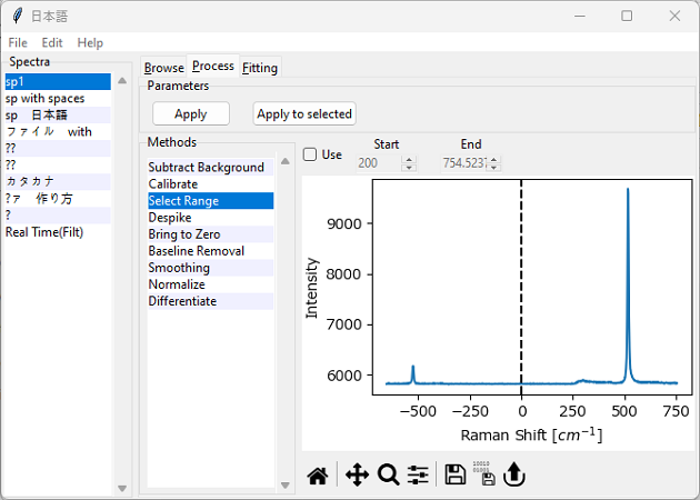
Fig. 4.2 The Preprocessing Window (Individual Spectra)

Otherwise, the preprocessing workflow outlined in Remarks on Processing Datasets applies to individual spectra as well.

4.2. Background Subtraction

Background subtraction refers to the process of removing an experimentally determined background signal from the dataset.

This is typically relevant in two scenarios:

• There is significant, non-random detector noise, e.g. different noise levels at different pixels of the CCD or InGaS detector.

• The signal is measured on top of a large background signal, for example originating from the sample substrate, that stays constant throughout the experiment. An example would be a thin biological specimen measured on a glass substrate.

See also

• To learn how to remove a non-constant background signal from the dataset (e.g. a fluorescent background), please see the Section on Baseline subtraction.

• To learn how to remove random noise from your dataset, please see the Sections on Smoothing and Denoising.

• If the desired signal is not entriely overwhelmed by the background and the dataset contains spectra of the background only, Automated Image Formation can often seperate background signal from the other spectral components.

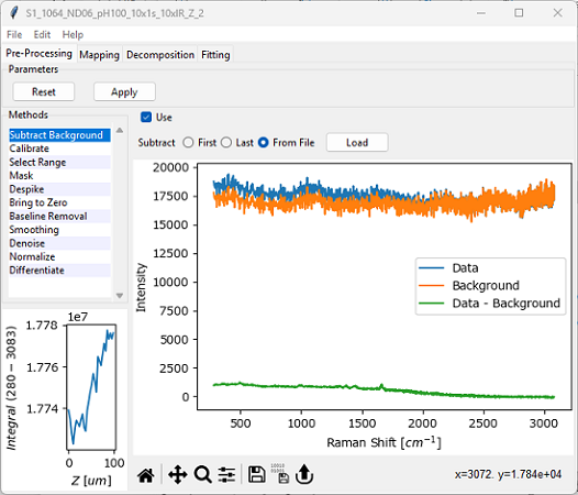
Fig. 4.3 The Background Subtraction Window

Parameters

Subtract

The experimental background signal to subtract from the dataset. Options are:

• First: The first spectrum of the dataset (e.g. t=0 for a time scan) contains the background and will be subtracted from all other spectra.

• Last: The last spectrum of the dataset will be subtracted from all other spectra.

• From File: Load a background spectrum from disk to subtract from the dataset. Supported file types are:

  • .mdt spectral databases

  • .s1d files containing a single spectrum

  • .hdf5 multi-spectrum files (see HDF5 Multi-Spectrum Files)

Important

SMDExplorer attempts to validate the selected background spectrum and displays an error if the number of points or spectral range of the background and the spectral dataset are different. There are no checks, however, whether the background signal was acquired under suitable experimental conditions.

4.3. Calibration

Calibration allows to correct the spectral axis of the dataset, for example to correct for drift of the spectrometer during the experiment.

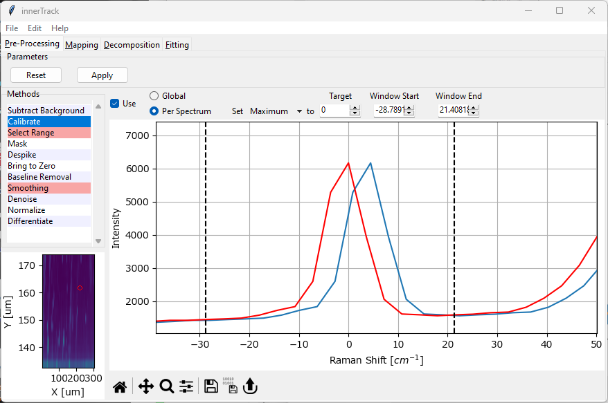
Fig. 4.4 The Calibration Window

Calibration (see The Calibration Window) provides two different modes:

• global calibration

• per spectrum calibration

The red spectrum in the graph in The Calibration Window displays the resulting spectrum.

4.3.1. Global Calibration

Here, a constant offset is applied to the spectral axis of each spectrum.

Parameters

Offset

The offset to apply to the spectral dimension (x-axis) of the dataset.

4.3.2. Per Spectrum Calibration

Here, a spectral feature (e.g. the maximum intensity in a certain spectral range) is set to a user-defined spectral position. The offset between the selected feature and the target value is calculated for each spectrum individually. This can compensate for spectrometer drift during an experiment but also provides a convenient way to offset spectra if the position of a peak is known with high accuracy.

Parameters

Method

The feature of the peak to use for the position calculation. This can either be the peak maximum (the default) or the peak centroid (center of mass).

Target

The target position of the peak. The default is zero, which is useful if the Rayleigh peak is present in the dataset.

Window Start

The start of the spectral region of interest. This can be set either by dragging one of the range selection lines in the graph or by typing a number into the Start box.

Window End

The end of the spectra region of interest.

Per spectrum calibration works by computing the selected parameter \(\rm{x}\) (maximum or centroid) across the window selected by Window Start and Window End. The offset is then calculated as \(\rm{\Delta x = x - x_{target}}\) and applied to each spectrum.

4.4. Range Selection

The Range Selection window allows selecting a (spectral) subrange of the acquired spectra for subsequent analysis, for example a certain range of wavenumbers for Raman spectra.

Typical applications are

• eliminating parts of the spectrum than contain no data (e.g, the range > 4000 cm^-1 for Raman spectra or the anti-Stokes region < 0 cm^-1).

• removing parts of the spectrum that are masked by filters in the optical setup.

• cropping the dataset to a region of interest for subsequent analysis, such as Automated Image Formation or Peak Deconvolution

• reducing the size of the dataset to speed up or facilitate subsequent processing steps.

• masking (strong) peaks that are of no interest for (or often detrimental to) further analysis, e.g. strong pump laser signals.

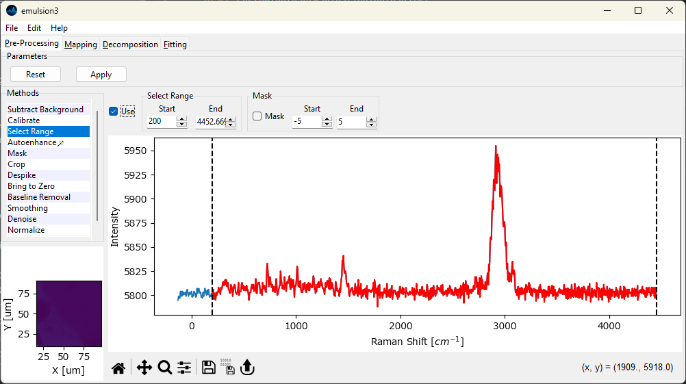
Fig. 4.5 The Range Selection Window

Parameters

Start

The start of the spectral region of interest. This can be set either by dragging one of the range selection lines in the graph or by typing a number into the Start box.

End

The end of the spectra region of interest.

The selected region is displayed in red in the graph (see The Range Selection Window).

Hint

Cropping the spectrum to the region containing only relevant spectral features can help the algorithms in Automated Image Formation converge significantly faster. In addition, removing instrumental artifacts, such as steps originating from edge or notch filters, facilitates further processing steps, in particular Basline Subtraction.

Mask

Mask a region at the center of the spectrum

Start

The start point of the excluded region

End

The end point of the excluded region

The masked region is indicated by a grey rectangle (Figure 4.6). Data in the masked region is replaced by a linear interpolation between the start end end points.

Note

Masking can be use to remove strong signals, e.g. the pump laser signal in Brillouin spectroscopy, to facilitate subsequent (semi-automated) analysis, in particular statistical denoising and automated image formation. Since these procedures rely on the relatve intensities of peaks, the pump laser signal, which can fluctuate strongly and is often orders of magnitude stronger than the signal originating from the sample, will dominate the variance of the dataset and lead to unsatisfactory results if the dataset is used naively.

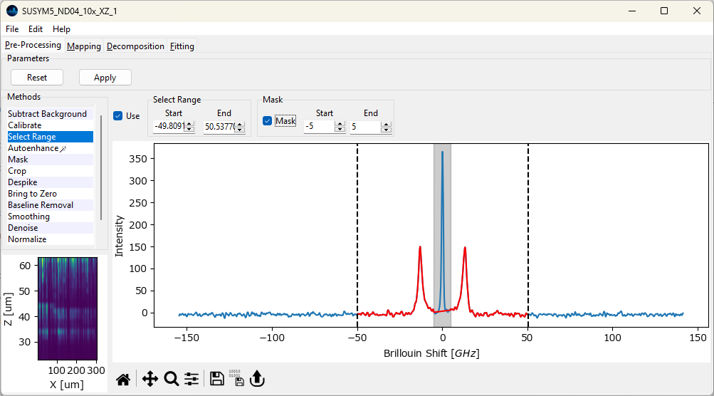
Fig. 4.6 Masking data.

During masking, data in the masked region is replaced by a straight line connecting the start and end points of the masked region (Figure 4.6). Masking of a central spectral region can also be performed during peak deconvolution without modification of the dataset. In this case, the contribution of the masked region to the mean-square error of between fit and data is reduced for the masked region, so that this region is effectively ignored during the fit.

4.5. Cropping

The spatial / temporal axes of spectral can be cropped to a region of interest to analyze only a subset of the acquired data.

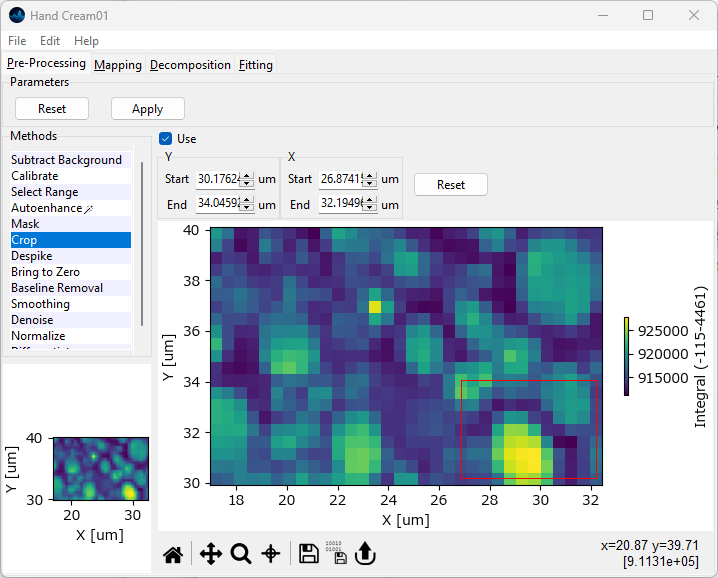
Fig. 4.7 The Cropping Window

Cropping can be accessed by selecting the Crop item from the sidebar of the Preprocessing tab.

Typical applications include:

• cropping a spatial scan to a region of interest.

• extracting segments from a temporal scan.

Cropping can also be used in tandem with Range Selection to trim the dataset for 3D display, for example in 3D or waterfall plots.

Parameters

Start

The start value of the cropping region for the respective dimension. The default value is the first datapoint of this dimension.

End

The final value of the cropping region for the respective dimension. The default value is the last datapoint of this dimension.

Reset

Resets the start and end values to the endpoints of the respective dimension.

Tip

Cropping can also be performed by dragging in the spectral mapping shown at the bottom of the panel. The limits in the top bar wil be adjusted automatically.

4.6. Cosmic Ray Removal (Despiking)

Cosmic rays are high energy particles originating form outer space that, when hitting the array detector of your spectrometer, result in sharp spikes in Raman spectra. These cosmic ray artifacts can interfere with downstream analysis of spectral datasets, in particular due to their high intensity when compared to the signal originating from the sample. While it is possible and desirable to minimize cosmic ray artifacts during data acquisition, it is often unavoidable to remove cosmic ray spikes from existing datasets as a preprocessing step during analysis.

Note

The detrimental effect of cosmic rays is mainly due to their high intensity, which is often orders of magnitude higher than the actual signal. This will significantly interfere with techniques that are sensitive to (or entirely rely on) absolute intensity, for example image formation based on the integrated intensity across a spectral range. Other techniques, such as automated image formation based on decomposition, are less sensitive to cosmic ray artifacts as long as the artifacts are infrequent in the dataset, which is typically the case.

In SMDExplorer, cosmic ray removal is achieved using the Despike preprocessing step (see The Despike Window).

See also

Masking can be used as an alternative to or in tandem with Despiking to exlude spectra affected by cosmic ray artifacts.

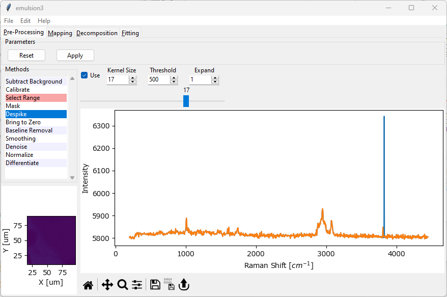
Fig. 4.8 The Despike Window

Parameters

Kernel Size

The window size of the median filter applied to the dataset. This should be an odd number. Use lower values to more sensitively detect spikes and higher values to decrease sensitivity.

Threshold

The minimum height (above the spectral baseline) above which to consider a spike a cosmic ray. Use lower values for increased sensitivity and higher values to detect only very high-intensity spikes.

Expand

The size of area around the cosmic ray to replace with the despiked signal. Use 1 (the default) to replace the minimum area around the detected spike and higher values to replace a wider spectral range. This parameter should be increased if Kernel Size is small to effectively remove high-intensity spikes.

For a detailed discussion of the three parameters, see Outline of the Algorithm.

When either parameter (Kernel Size, Threshold, Expand) is changed, the entire dataset is re-checked for cosmic ray artifacts. Depending on the size of the dataset, this can take a significant amount of time. Cropping the spectral range using Range Selection can speed up analysis. The slider in the Despike window allows scrolling through the spectra with detected cosmic rays to check successful despiking.

4.6.1. Outline of the Algorithm

Cosmic ray detection and removal in SMDExplorer involves a two stage algorithm.

        flowchart LR
    in[Input]-->A

    subgraph  diff [Difference Spectrum]

    A[Spectrum S] -->|median filter| B(filtered F)
    
    A & B-->C{"S-F"} --> D[Difference Spectrum D]
    end

    D --> XX{Threhold}

    A & XX -.->|D < threshold| EE[" "]-.-> E(Output)
    XX-->|D > threshold| F
    subgraph spike [Despike]
    F(Cosmic Ray Candidate)

    F & A  -->|Peak Finding| G{{Cosmic Ray Regions R}}
    G & B & A-.-> H[Fill R with Filtered]
    
    end

    H --> E
    

Fig. 4.9 The Cosmic Ray Detection Algorithm

1. Median filtering of the input spectrum \(S\) using Kernel Size as the window size for the computation of the sliding median resulting in spectrum \(F\) (see Cosmic Ray Filtering - Kernel Size bottom).

2. Computing the difference spectrum \(D = S-F\) (see Cosmic Ray Filtering - Kernel Size top).

3. Thresholding the difference spectrum \(D\) using the Threshold parameter.

   • if \(D < threshold\), the spectrum contains no cosmic ray artifacts and is left unaltered.

   • if \(D > threshold\), the spectrum contains cosmic ray artifacts that will be removed by replacing the spike with the median filtered signal.

4. Use peak detection to identify the segments of the spectrum affected by cosmic ray artifacts.

5. Replace the cosmic ray segments by the median-filtered spectrum \(F\). The size of the detected segments can be expanded by the Expand parameter as needed (see Cosmic Ray Filtering - Expand).

6. Return the filtered spectrum.

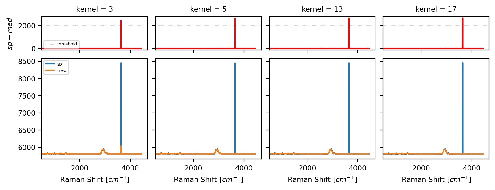
Fig. 4.10 Cosmic Ray Filtering - Kernel Size

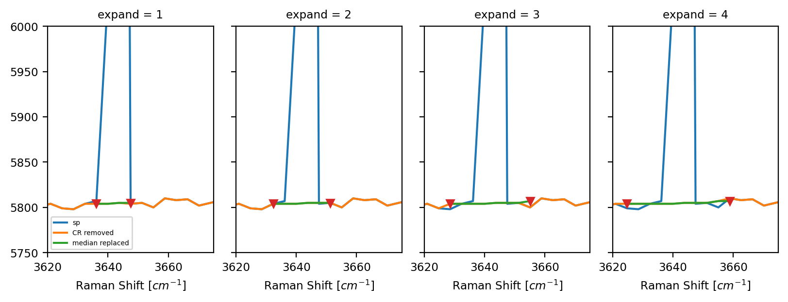
Fig. 4.11 Cosmic Ray Filtering - Expand

4.7. Simple Baseline Removal (Bring to Zero)

Simple Baseline Removal allows the subtraction of an offset from the spectral dataset. This can be used to bring the baseline spectra in your dataset to zero.

Simple Baseline Removal works by computing the arithmetic mean of a selected spectral region and subtracting this mean from the spectrum. This is done for each spectrum individually to account for potential drift of the baseline during the experiment. In a typical use case, the selected spectral region contains no spectral features (i.e. noise only).

See also

• for removing a non-constant baseline from your dataset (e.g. a fluorescent background), see Non-linear Baseline Removal.

• to subtract an exerimentally determined background spectrum, see the section on Background Subtraction.

• Typical fluorescent background is also efficiently eliminated using 2^nd derivative spectra.

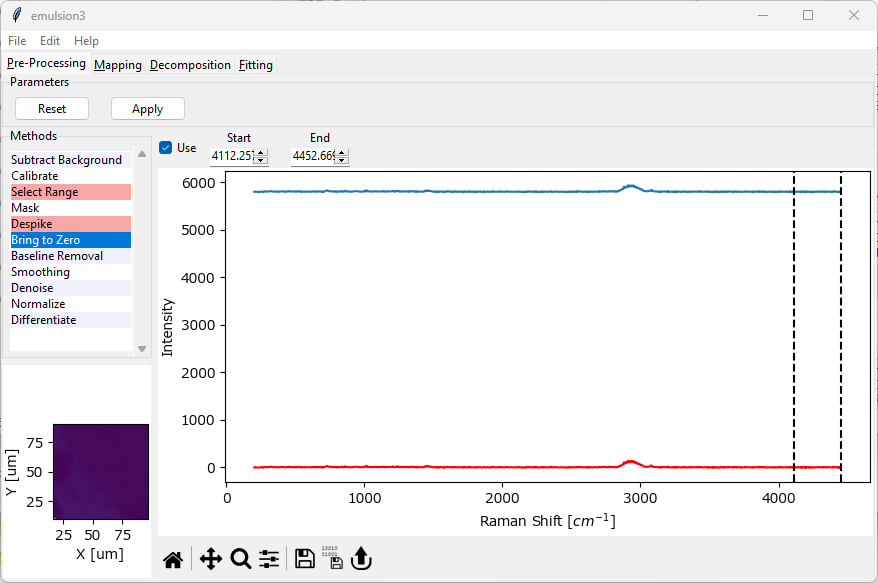
Fig. 4.12 The Bring-To-Zero Window

Parameters

Start

The start of the spectral region of interest. This can be set either by dragging one of the range selection lines in the graph or by typing a number into the Start box.

End

The end of the spectra region of interest.

The mean between Start and End will be subtracted from the spectrum. The resulting spectrum is displayed in red in the graph (The Bring-To-Zero Window).

Note

The algorithms in Automated Image Formation are typically not scale invariant, which means that the absolute magnitude of the signal affects the solution of the spectral decomposition. Consequently, emphasizing the spectral features by setting the background to zero after baseline subtraction is recommended to help the algorithm find useful solutions.

4.8. Non-linear Baseline Removal

Non-linear Baseline Removal allows the subtraction of a non-constant, fluctuating baseline from the dataset, for example a fluorescent background. SMDExplorer implements the Statistics-sensitive Non-linear Iterative Peak-clipping (SNIP) algorithm (Ryan, 1988).

The baseline will be computed for and subtracted from each spectrum individually to account for effects like photobleaching, etc.

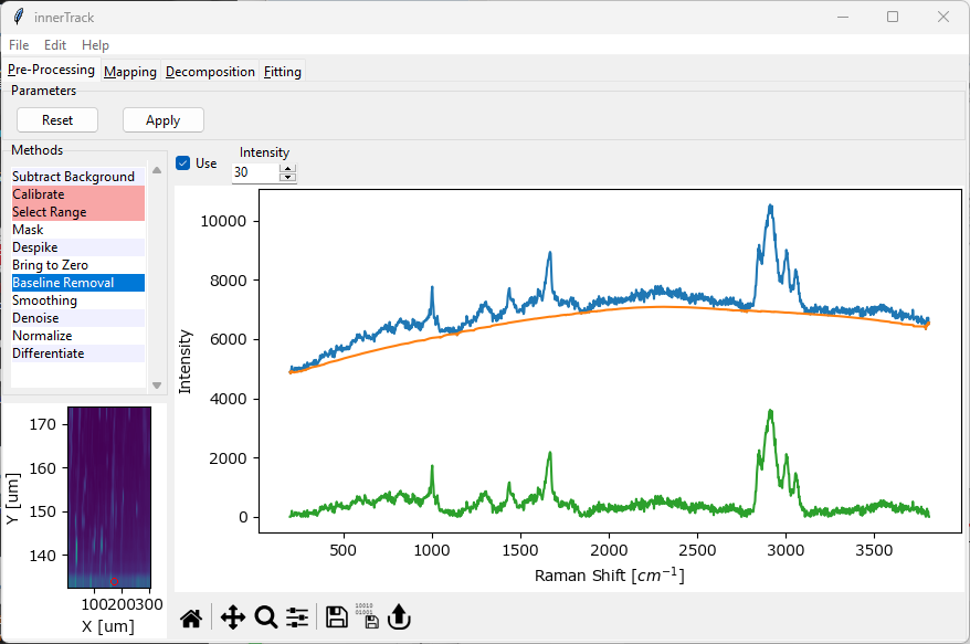
Fig. 4.13 The Baseline Subtraction Window

Parameters

Intensity

The number of passes of the peak clipping loop. Use a lower number to allow regions of higher curvature in the baseline and a higher number for a smoother baseline (see the orange traces in Baseline Subtraction - Intensity). A good starting value is 30 (the default).

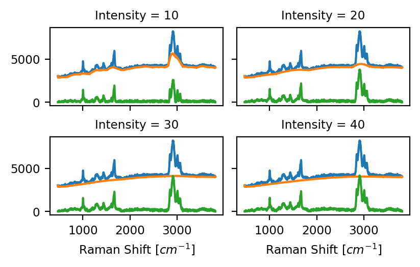
Fig. 4.14 Baseline Subtraction - Intensity

Note

The algorithms in Automated Image Formation are typically not scale invariant, which means that the absolute magnitude of the signal affects the solution of the spectral decomposition. Consequently, emphasizing the spectral features by setting the background to zero by baseline subtraction is recommended to help the algorithm find useful solutions.

4.9. Smoothing

Smoothing refers to the process of removing noise from individual spectra of your dataset. If your dataset consists of several related spectra, for example measured during a time scan or a spatial mapping, Denoising can be used in addition or as an alternative to Smoothing to remove noise.

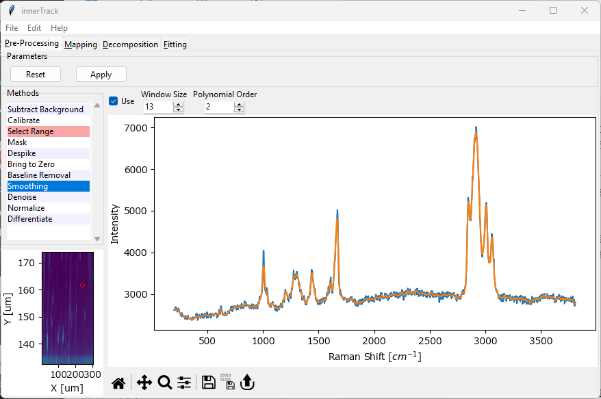
Fig. 4.15 The Smoothing Window

SMDExplorer implements three smoothing methods:

• Savitzky-Golay smoothing (Savitzky & Golay, 1964). Savitzky-Golay smoothing involves fitting adjacent data points with a low-degree polynomial.

• windowed Savitzky-Golay smoothing (Schmid, 2022)

• Whittaker smoothing (Eilers, 2003)

Parameters

Method

Selects the smoothing algorithm. Depending on the selected method, a number of parameters can be adjusted:

Window Size (Savitzky-Golay)

The size of the smoothing window, i.e. the number of data points to fit (see Figure 4.16). This should be an odd number. Higher values will lead to more noise removal but can result in signal distortion (e.g. peak shifts).

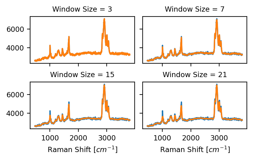
Fig. 4.16 Savitzky-Golay Window Size (Polynomial Order 2)

Polynomial Order (Savitzky-Golay)

The degree of the polynomial to fit the data (see Figure 4.17). A higher-degree polynomial will result in a better fit (less distortion) but also lower noise reduction.

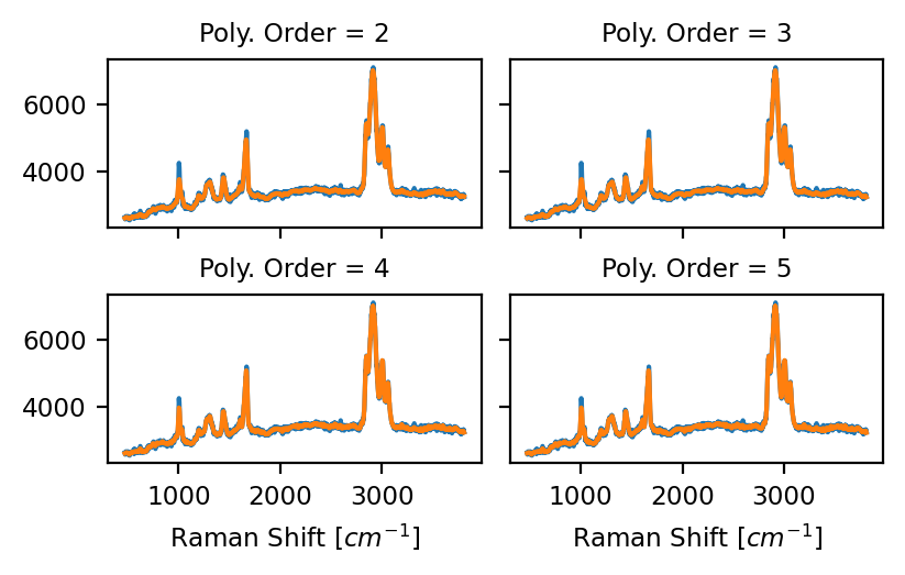
Fig. 4.17 Savitzky-Golay Polynomial Order (Window Size 15)

Lambda (Whittaker smoothing)

Selects the smoothing parameter \(\log(\lambda)\) of the Whittaker smoother. Higher values result in more smoothing.

Note

For a detailed discussion on the merits of the individual algorithms, see Schmid, 2022 and Figure 4.18.

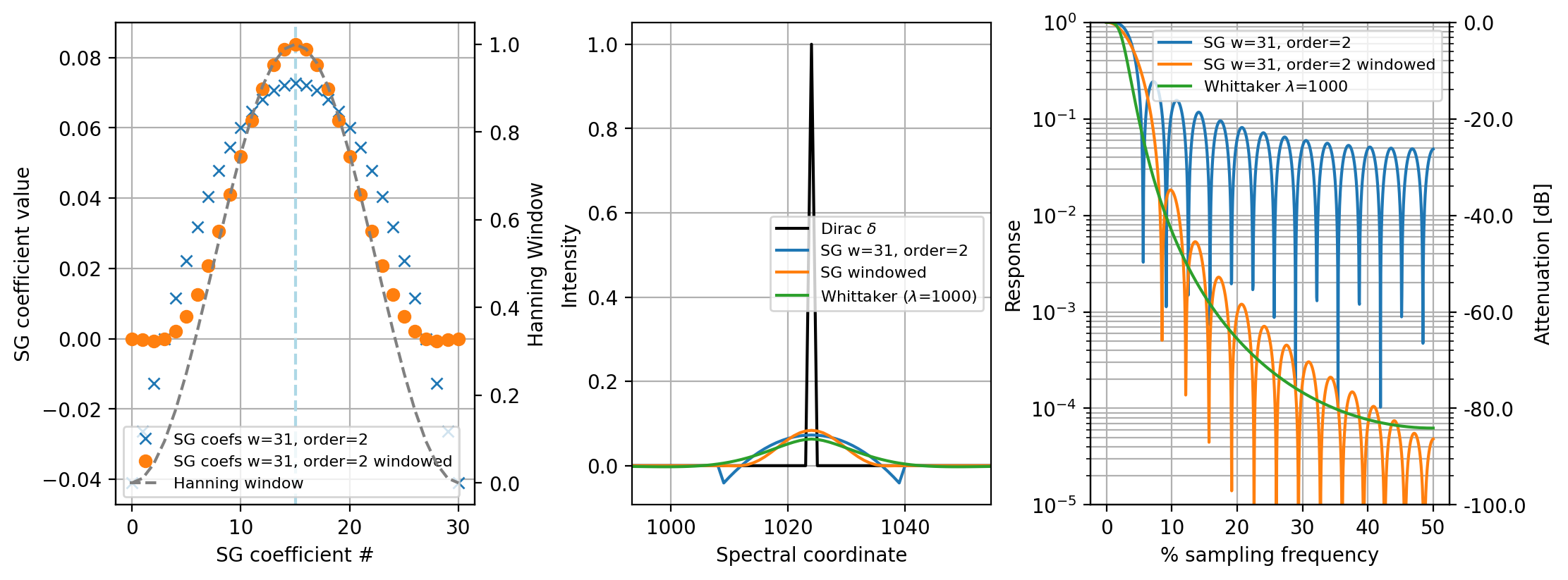
Fig. 4.18 Left: applying a window to the Savitzky-Golay coefficient reduced boundary artifacts. Center: Comparison of the three smoothing algorithms on an impulse function. Right:Frequency response of the three filters.

For experimental data, the three methods can mostly be used interchangably (Figure 4.19).

Comparison

Comparison (zoom)

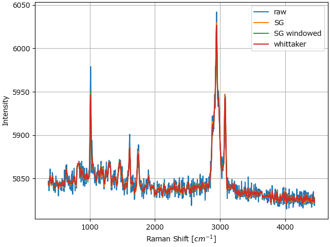
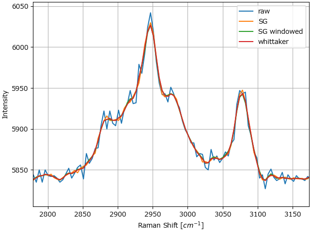
Fig. 4.19 Comparison between the smoothing filters on a Raman dataset.

4.10. Averaging / Binning / Denoising

Denoising refers to the process of removing noise from the data by taking advantage of several spectra obtained from the same (or a closely related) sample in succession, for example during a spatial mapping or a time scan. Here, the assumption is that noise will fluctuate randomly while the signal remains constant. This allows noise removal by statistical procedures, e.g. averaging in the simplest case.

See also

• To remove noise from individual spectra, please see the Smoothing section.

• To remove non-random noise from a dataset, see the Background Subtraction section.

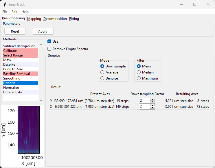
Fig. 4.20 The Denoise Window

Parameters

Remove Empty Spectra

When this option is checked, empty spectra (spectra that are entirely zero) will be removed from the dataset before applying the selected denoising algorithm.

Mode

The Denoising Method. See the sections below for a discussion of the individual methods and their parameters.

See also

Empty spectra can also be removed using masking (see the Masking Section). Masking allows more fine-grained control over which spectra to omit.

SMDExplorer implements three different denoising methods:

• Denoising by downsampling. Here, spectra are averaged across a user-defined window for each dimension and the size of the dataset is reduced by the size of the window. This is also often referred to as Pooling or Binning. This mode is activated by the Downsample radio button.

• Denoising by averaging. Here, spectra are (again) averaged across a user-defined window but each spectrum is replaced by the sliding average. The size of the denoised dataset is, accordingly, identical to the original dataset. This mode is activated by the Average radio button.

• Statistical denoising. Here, the dataset is first transformed using a dimensionality reduction method (e.g. PCA) into a sparse representation of the dataset. The original dataset is then reconstructed from this sparse representation, effectively reducing noise. This mode is activated by the Denoise radio button.

The three denoising methods will be discussed in detail in the following sections.

Important

While the effect of the Downsampling and Averaging denoising filters is easily visualized using two-dimensional images, please keep in mind that these filters are not image filters. They rather operate on the entire hyperspectral dataset and denoise the spectra that are then used to form the images.

4.10.1. Denoising by Downsampling

Downsampling involves dividing the dataset into bins and replacing the data of the bin by an aggregate spectrum (computed by a function that acts on the entire bin). This decreases the size of the dataset by a factor (in the one-dimensional case) of \(\rm{1/binSize}\) (see The Downsample filter). In SMDExplorer, this parameter is determined by the Window Size parameter, which can be set independently for each dimension of the dataset. The resulting dimensions are automatically computed.

Hint

While downsampling can in principle be performed for any Window Size, optimal downsampling (i.e. no boundary effects) can be achieved if Window Size is a divisor of the corresponding dimension of the original dataset.

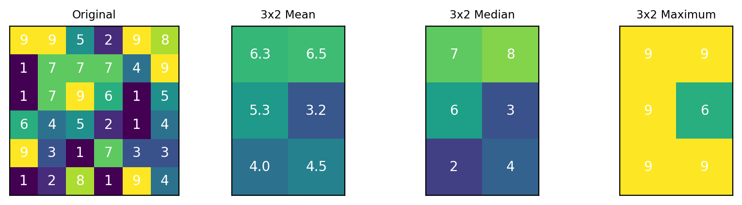
Fig. 4.21 The Downsample filter

The following functions are available for computing the resulting downsampled spectrum:

• arithmetic mean

• median

• maximum

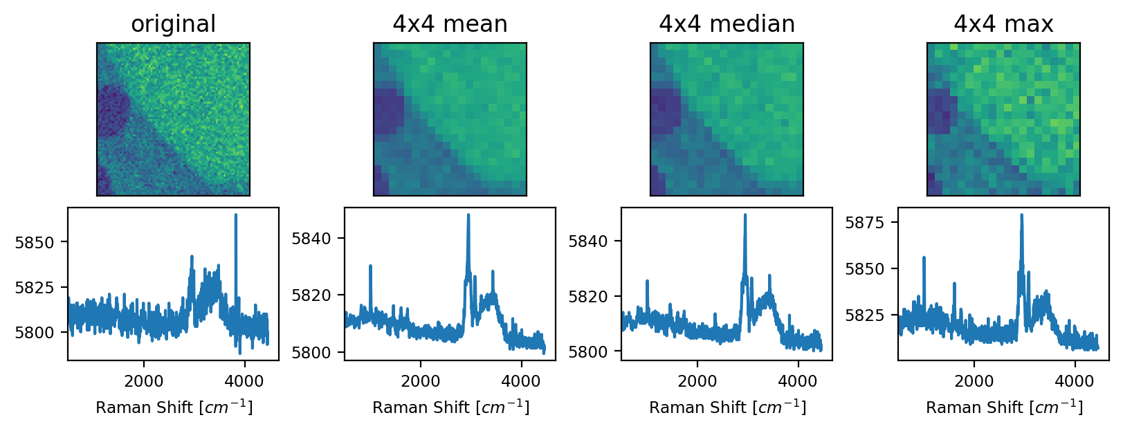
Fig. 4.22 The Downsample filter - An example

The arithmetic mean filter has the strongest smoothing effect results in blurring of spatial features, in particular sharp edges, of the dataset in The Downsample filter - An example. The median filter is edge-preserving, so sharp transitions in the original dataset are preserved at the expense of reduced noise removal. The Maximum filter replaces each bin by the maximum spectrum in the bin, which does not, per se, denoise the data but can enhance the signal-to-noise ratio.

Hint

Downsampling can be be used to collapse entire dimensions, for exaple to convert an XZ-scan to a one-dimensional Z-scan by computing an aggregate spectrum across one dimension or to compute the mean spectrum of a time series.

4.10.2. Denoising by Averaging

During averaging, a window is moved across the dataset and the spectrum at the center of the window is replaced by an aggregate spectrum computed across the window (The Average filter). This preserves the size of the original dataset.

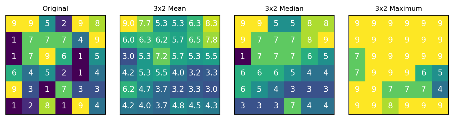
Fig. 4.23 The Average filter

The following functions are available for computing the aggregate spectrum:

• arithmetic mean

• median

• maximum

• total variation (Chambolle, 2004)

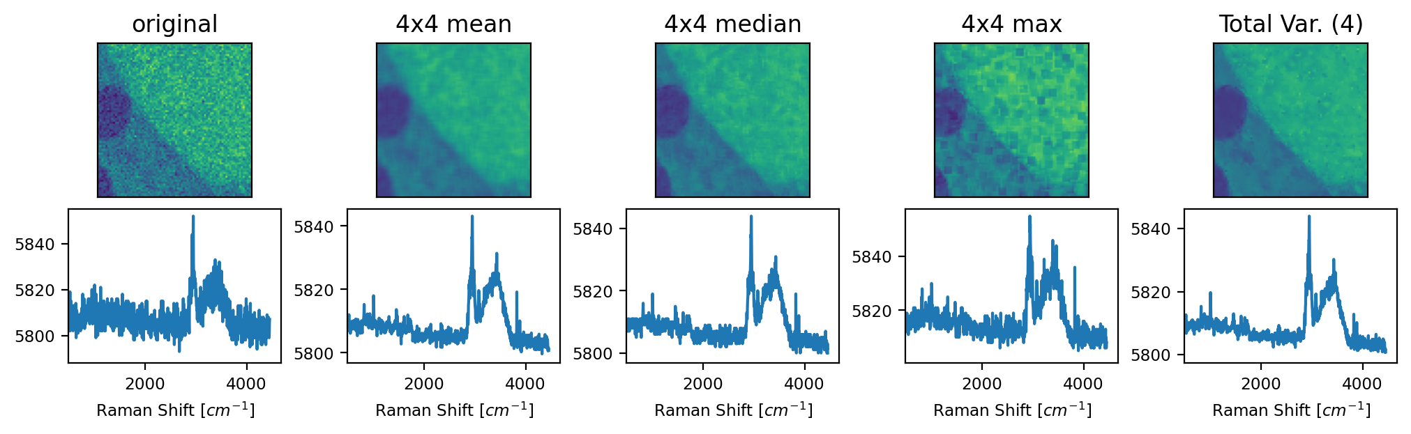
Fig. 4.24 The Average filter - An Example

For a discussion of the arithmetic mean, median, and maximum filters, see the Denoising by Downsampling section. The Total Variation filter results in a high degree of averaging (strong denoising) in regions with similar spectra and lower averaging in regions with higher spectral variance. This leads to strong denoising while preserving edges and small details (see The Average filter - An Example).

Note

The Total Variation filter only accepts one input parameter. For denoising, the Window Size of the first dimension is used.

4.10.3. Statistical Denoising

Statistical denoising consists of finding a sparse representation of the dataset, which contains the essential features of the spectra but little noise, and reconstructing a denoised dataset from this sparse representation. SMDExplorer implements three statistical denoising algorithms, denoising by Principal Component Analysis (PCA), denoising by Maximum Noise Fraction (MNF), or denoising by Smooth Factor Analysis (SFA).

Note

Since Statistical Denoising does not operate along any (spatial or temporal) dimensions of the dataset, there is no risk of blurring edges.

The key factor for statistical denoising is the size of the dataset. Even if individual spectra have a low or mediocre signal-to-noise ratio, statistical denoising will efficiently extract the relevant spectral characteristics from the dataset and remove noise provided that the characteristic spectral signature appears frequently enough. It is hence possible to employ low exposure times or low laser power (to reduce sample damage) and / or fast scanning rates (to increase spatial resolution) and to recover the signal by denoising during data processing.

Note

Statistical denoising relies on the fact that the desired signal appears more frequently in the dataset compared to (randomly distributed) noise; in other word, the signal has a higher contribution to the variance of the data. Unfortunately, this entails that the statistcial denoisng algorithms are not scale invariant - strong signals tend to dominate the variance of the dataset, which can result in poor denoising performance if the dataset contains signals with intensities that strongly vary in magnitude.

This can lead to:

• small signals being eliminated entirely, which is (luckily) readily detectable.

• small signals being retained, but, since their contribution to the overall variance is low, variations (e.g. changes in intensity or position of spectral peaks) of the small signals are reduced or eliminated. While denoising performance is (superficially) satisfactory, the overall variability of the dataset is artificially reduced, and many spectra will essentially be identical. This is a subtle effect that can be hard to detect (Figure 4.25).

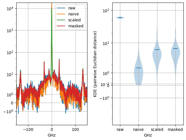
Fig. 4.25 Variability reduction by statistical denoising in spectral dataset with signals that span many orders of magnitude. The left panel shows a spectrum with a signal of interest of between 10 to 100 counts and a central peak of 10000 counts. Naive PCA denoising efficiently removes noise but also strongly reduces (scientifically meaningful) spectrum-to-spectrum variations (right panel), with many spectra being completely identical. This effect can be avoided by either masking the central peak or compressing the dynamic range of the dataset using LLS scaling.

This issue can be circumvented by several means:

• if the strong signals are of no interest for subsequent analysis, they can be removed by Range Selection and (internal) masking.

• spectra with strong signals can be exluded from analysis entirely.

• if the strong signals are cause by cosmic ray artifacts, they can be removed by despinking.

• the dataset can be (reversibly) scaled to compress the dynamic range, effectively reducing the effect of the high-intensity signals. In SMDExplorer, this is achieved by Log-Log-Square (LLS) scaling (4.1).

  (4.1)\[ V(i) = \log{ \left[ \log{\left( \sqrt{ y(i)+1}+1\right)}+1\right]} \]

  LLS scaling can be activated using the LLS scale data checkbox.

Denosing performance (in terms of SNR gain) is typically similar for scaled and unscaled data as statistical denoising relies on both intensity and frequency of occurence to remove noise (Figure 4.26).

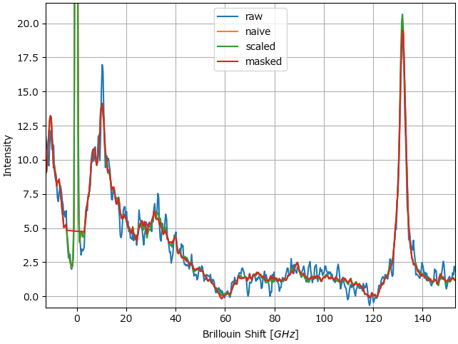
Fig. 4.26 PCA denoising performance comparison.

Using scaling or (internal) masking is of particular relevance for denosing datasets of Brillouin spectra, where the pump laser signal intensity (at the center of the spectral range) can fluctuate by several orders of magnitude.

4.10.3.1. PCA Denoising

For PCA denoising, we take advantage of the fact that the principal components are ordered in descending order of explained variance, which means that the first few components contain most of the variance (i.e. relevant signal) of the dataset while the higher order components contain spurious noise and other artifacts (see PCA Denoising). By reconstructing the dataset from the sparse representation containing only the first few components, noise and other artifacts (e.g. cosmic rays) will be removed from the denoised dataset (see PCA Denoising - An example).

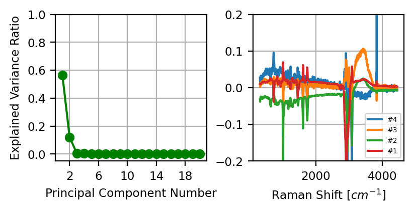
Fig. 4.27 PCA Denoising

See also

For a detailed discussion of dimensionality reduction, including PCA, also see the Automated Image Formation Section.

The number of components, which, in SMDExplorer, defaults to 8, should be set appropriately for the spectral dataset under investigation. A smaller number of components results in strong denoising but carries the risk of missing essential spectral components, especially if there are a number of very different spectra in the dataset. Increasing the number of components will result in more noise and other artifacts in the reconstructed denoised dataset.

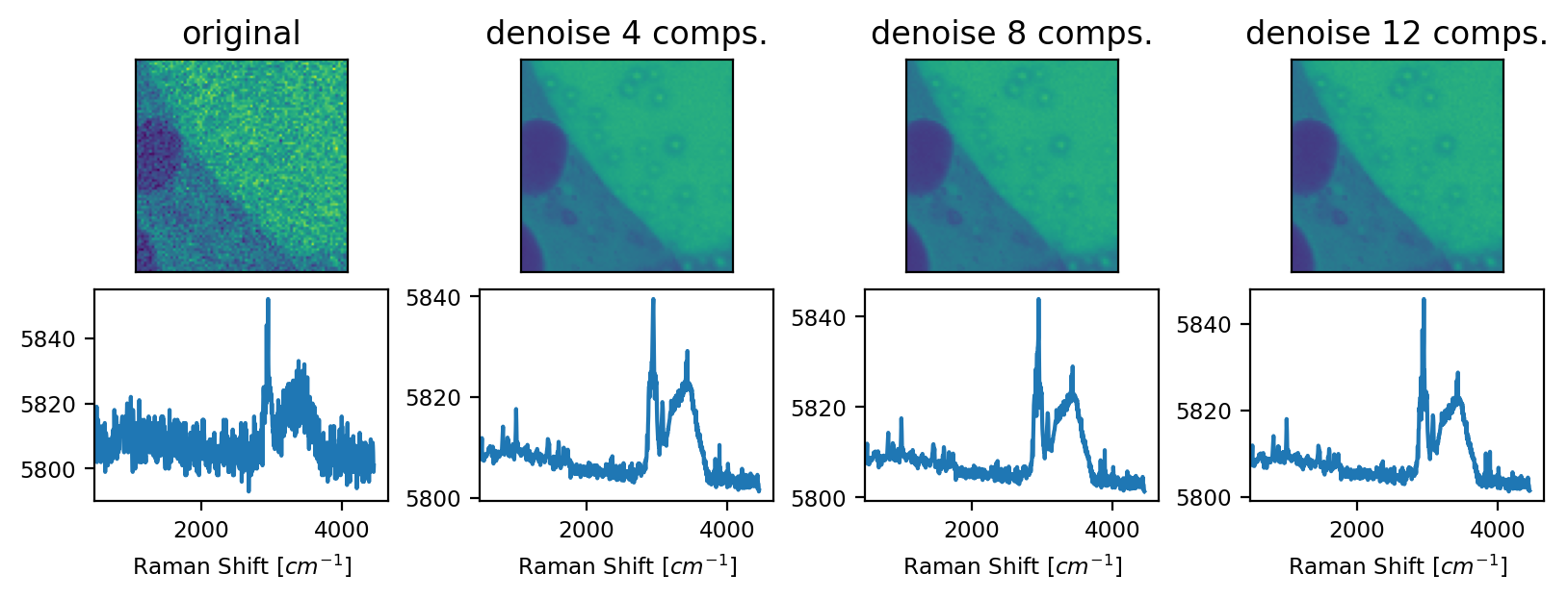
Fig. 4.28 PCA Denoising - An example

4.10.3.2. MNF Denoising

In Minimum Noise Fraction denoising involves two subsequent PCA transformations to compute the linear combination of components that maximizes the signal-to-noise ratio. To this end, the noise of the dataset is first estimated from the covariance matrix of the data, followed by noise whitening.

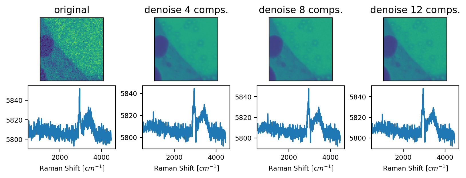
Fig. 4.29 MNF Denoising - An example

Hint

The choice between PCA or MNF depends on the noise characteristics of the dataset. Literature reports suggest that PCA performs better for random (Gaussian) instrument noise whereas MNF is preferable if noise levels vary across spectral channels, i.e. wavenumbers, or spatial locations. A good overview about different denoising techniques can be found in Jahn, 2021.

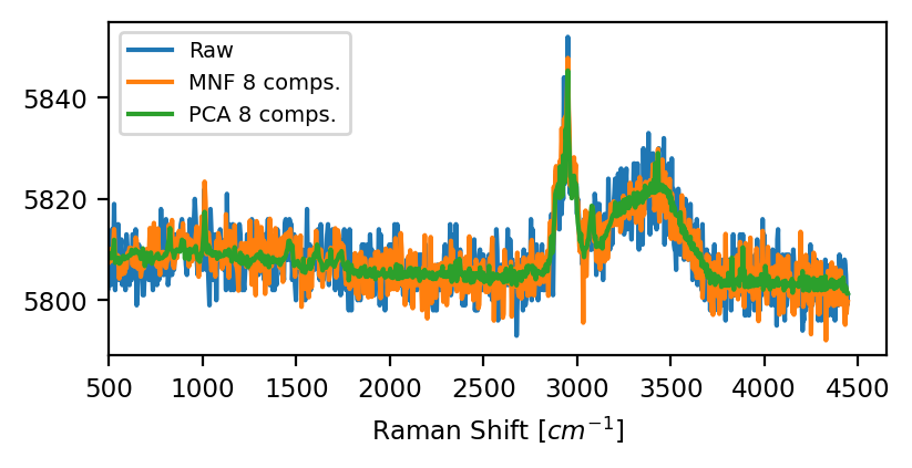
Fig. 4.30 PCA vs MNF denoising

4.10.3.3. SFA Denoising

Smooth Factor Analysis (SFA) (Park et al., Applied Spectroscopy. 2018;72(5):765-775.) combines smoothing with PCA denoising (see above).

In a nutshell, this procedure combines:

1. dimensionality reduction (like PCA) to exclude noise (which has (in the ideal case) an equal contribution to all extracted components) by reconstructing the dataset from a sparse representation containing only a few components (loading and score vectors) that have the biggest contribution to the variance. of the dataset (i.e. the signal).

2. Savitzky-Golay (SG) smoothing of the extracted loading vectors (spectra). Smoothing can be performed quite aggressively since distortions can be recovered by extracted downstream components.

By performing per-component smoothing on the loading vectors, a high degree of denoising can be achieved with minimal spectral distortion.

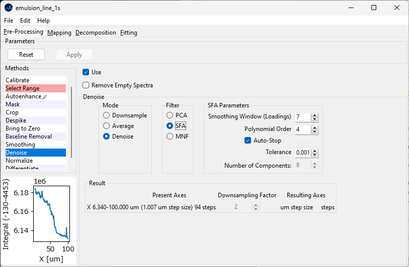
Fig. 4.31 The SFA denoising panel.

Parameters

Smoothing Window

The size of the smoothing window that is applied to the loading vectors. This parameter is equivalent to the Window Size parameter of Savitzky-Golay smoothing. A higher value will lead to more smoothing at the risk of greater distortion. The effect of this parameter can be seen in the bottom rows of Figure 4.32.

Polynomial Order

The order of the polynomial to fit to the data during the smoothing procedure. This parameter is equivalent to the of Savitzky-Golay smoothing. A higher value will lead to less smoothing and less distortion.

Auto-Stop

Terminates the extraction of components when the explained variance of the extracted component falls below the Tolerance value. Alternatively, the number of components to be extracted can be set manually.

Tolerance

Autostopping criterion - the minimum amount of explained variance of a newly extracted component until iterations stop

Number of Components

The number of (smoothed) components to use when reconstructing the dataset. This parameter is equivalent to the Number of Components parameter of PCA denoising. The effect of this parameter can be seen in the top rows of Figure 4.32.

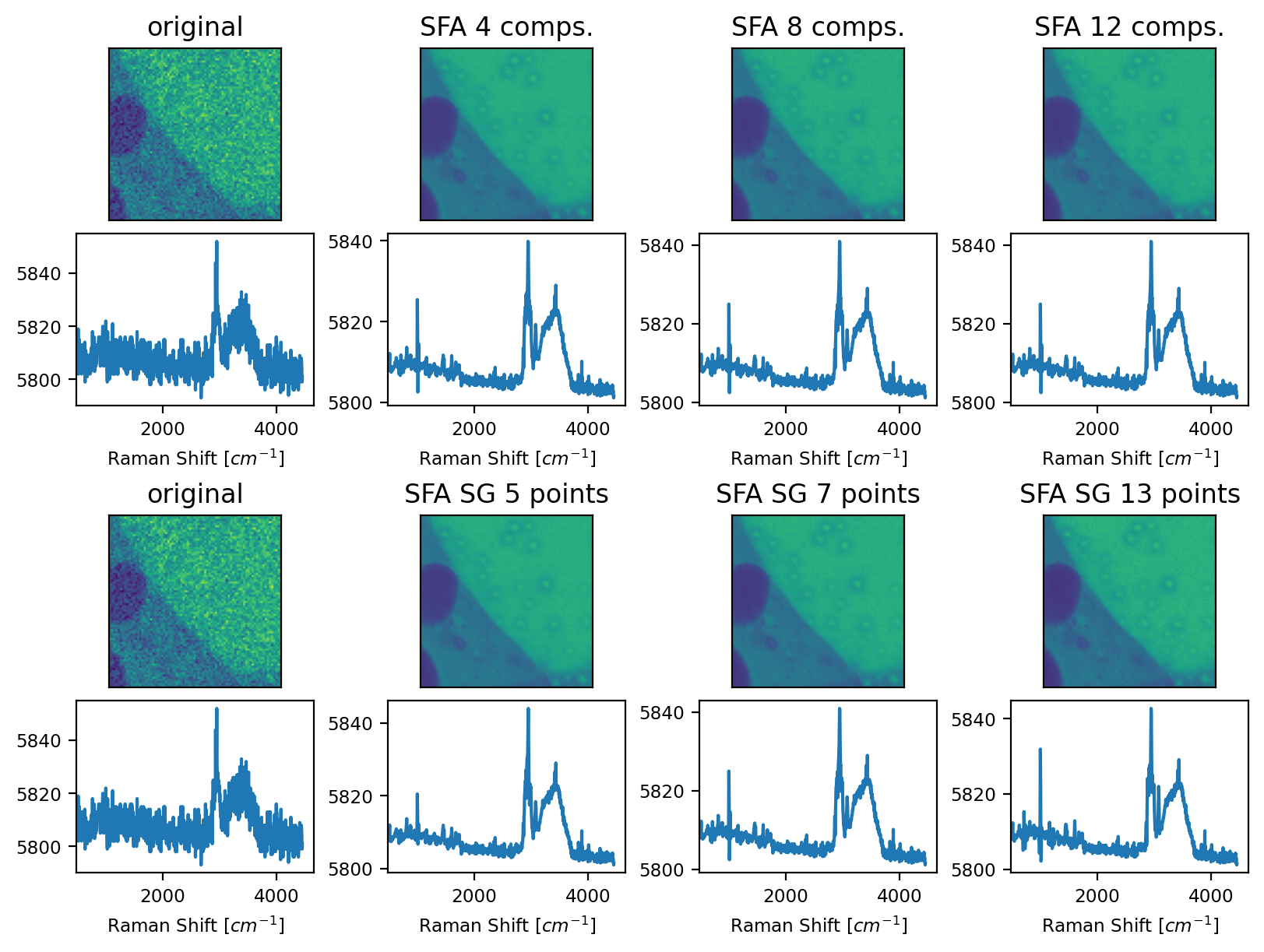
Fig. 4.32 SFA Denoising - An example

Note

The choice between PCA denoising and SFA denoising primarily depends on the size of the dataset. For small-to-medium size datasets (a few hundred spectra or less), the combined power of statistical and per-trace denoising of SFA will outperform PCA denosing for the same number of components. For (much) larger datasets, SFA denosing provides no additional benefit and the added computational cost (as well as the possible risk of spectral distortion) outweighs the minimal gain in signal-to-noise ratio.

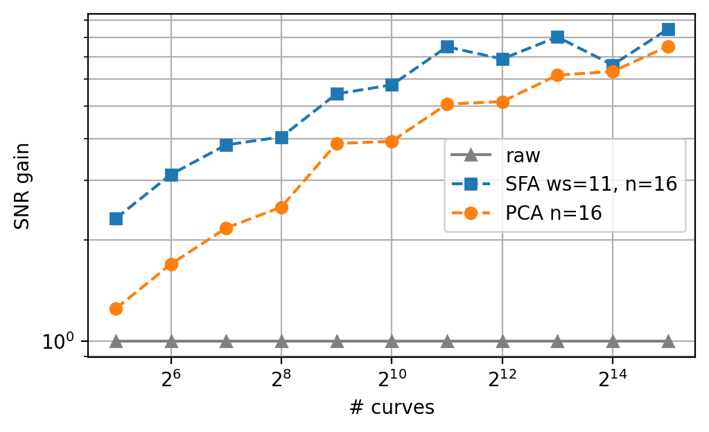
Fig. 4.33 PCA vs. SFA denoising - dataset size dependence.

When selecting the number of components, the same heuristics discussed for PCA denoising apply - a larger number of components increases the amount of noise remaining in the dataset but also increases reconstruction fidelity.

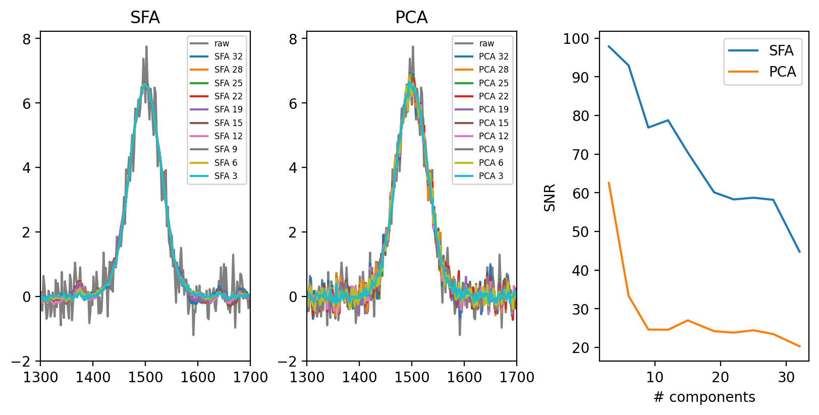
Fig. 4.34 PCA vs. SFA denoising for a dataset of 100 spectra - number of components.

Alternatively, the Auto-Stop parameter provides a convenient way to select an optimal number of components.

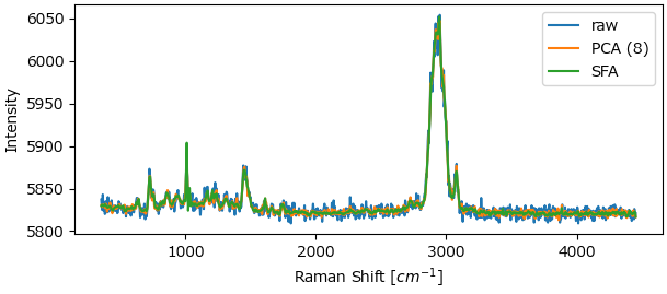
Fig. 4.35 PCA vs. SFA denoising on a real-world dataset (100 curves).

4.11. Normalization

Normalization can be used to compensate for intensity fluctuations in the dataset, for example due to focus drift or sample unevenness. Each spectrum is either normalized (i.e. divided) by the integrated intensity across a selected spectral region or scaled between 0 and 1. In typical use, this spectral region is expected to remain constant throughout the experiment.

See also

Normalization can also be performed by plotting the ratio of two spectral regions, see Intensity Profile Options in the Intensity Profiles / Image Formation Section.

Hint

It often makes sense to subtract a baseline before normalization. This can be achieved by subtracting a constant offset or a non-linear baseline.

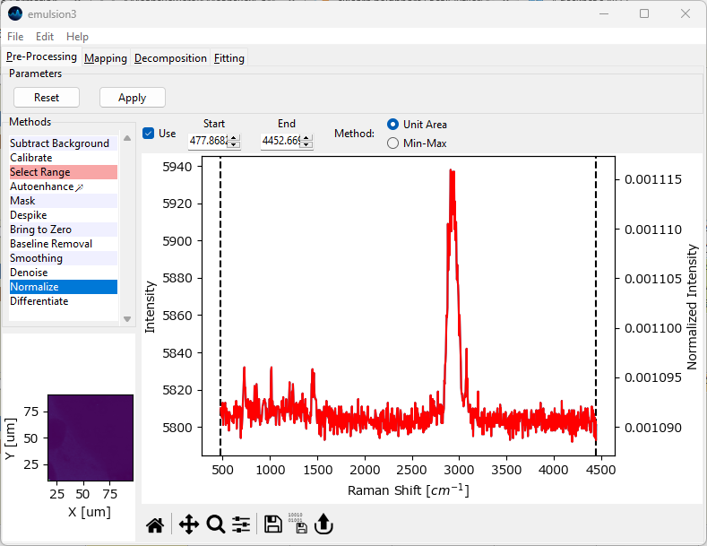
Fig. 4.36 The Normalization Window

Parameters

Start

The start of the spectral region of interest. This can be set either by dragging one of the range selection lines in the graph or by typing a number into the Start box.

End

The end of the spectra region of interest.

Method

The normalization method to apply:

• Unit Area: Each spectrum will be divided by the integrated intensity between Start and End, which will result in a spectrum with an integrated intensity of one.

• Min-Max: Scale the selected spectral region between 0 and 1.

By default, Start and End are set to include the entire spectral range. The red trace in the preview window displays the resulting spectrum, with the normalized intensity displayed on the right-hand vertical axis.

4.12. Differentiation

Differentiation allows the computation of the (numerical) 1^st and 2^nd derivatives of the spectra in a dataset (see The 1st and 2nd derivatives for a toy example involving a single Lorentzian peak).

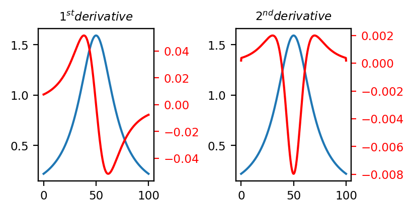
Fig. 4.37 The 1^st and 2^nd derivatives

Typical applications are:

• removal of a linear (1^st derivative) or polynomial (2^nd derivative) background from the data.

• separation of overlapping peaks (2^nd derivative).

See Easy Visualization using Derivatives for a visualization. Computing the 2^nd derivative removes the parabolic baseline and nicely separates the two overlapping peaks (the 2^nd derivative trace has been multiplies by \(\rm{-1}\) to match the positive peaks in the original signal).

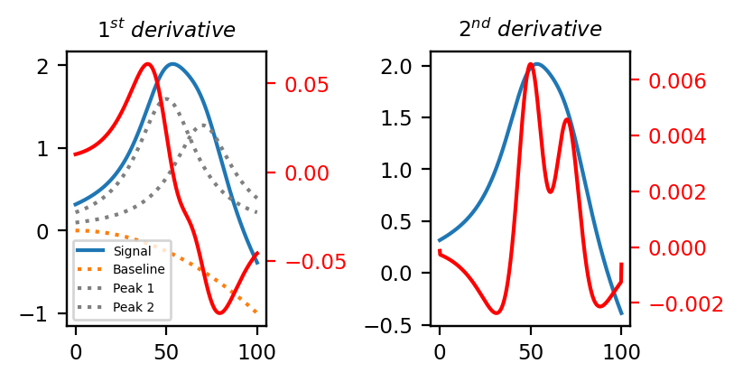
Fig. 4.38 Easy Visualization using Derivatives

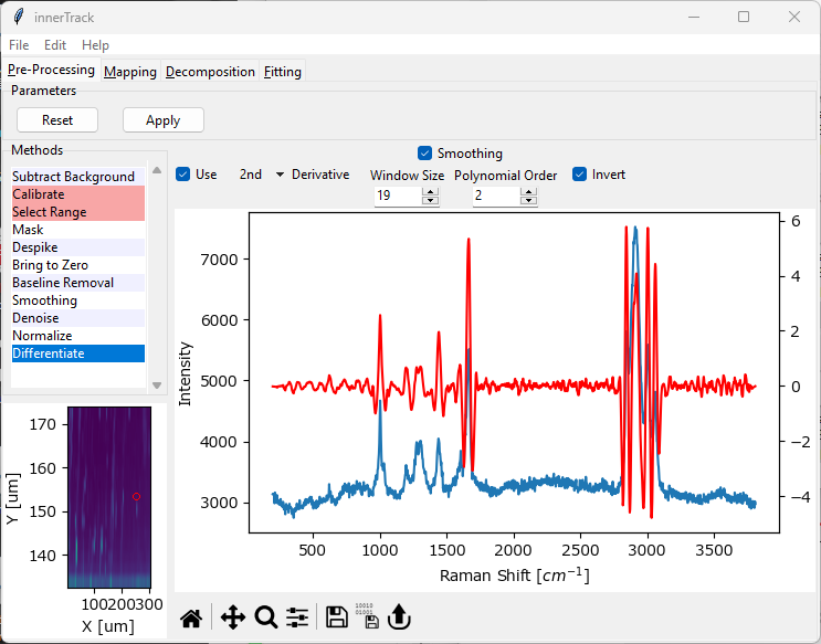
Fig. 4.39 The Differentiation Window

Parameters

Derivative Degree

Compute either the 1^st or 2^nd derivative of the dataset.

Smoothing

Apply Savitzky-Golay smoothing to the data before computing the derivatives to counter the effect of noise resulting from numerical differentiation. See the Smoothing Section for a discussion of Window Size and Polynomial Order.

Invert

Multiply the resulting spectra by \(\rm{-1}\). This will result in positive peaks in the original spectrum to appear as positive peaks in the 2^nd derivative spectrum as well.

Important

Numerical differentiation, especially successive steps of numerical differentiation, leads to a significant increase of noise in the dataset. Noise removal, either by Smoothing or Averaging / Binning / Denoising is crucial to eliminate spurious peaks that result from differentiation. On the other hand, smoothing should be used judiciously as to avoid artifacts resulting from smoothing, i.e. peak shifts.

4.13. Masking

Masking allows to exclude selected spectra from analysis and plotting based on their intensity. Typical applications include:

• removing blank spectra (spectra that contain only background or are zero entirely) from the dataset

• masking low-intensity or high-intensity regions for easier visualization of structures in spatial scans

• removal of high-intensity cosmic ray artifacts (see also the section Cosmic Ray Removal (Despiking) for despiking based on median filtering)

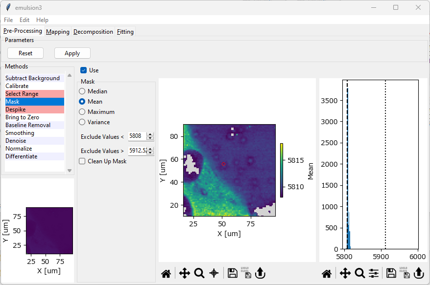
Fig. 4.40 The Masking Window

Masking works by computing an aggregate metric (e.g. the arithmetic mean) for each spectrum and excluding spectra that lie outside this metric. A mapping of this metric is shown in the center panel of The Masking Window. For easier visualization, a histogram (frequency distribution) of this metric is shown in the right panel of The Masking Window. The center mapping updates when the masking parameters are changed to illustrate which spectra are going to be excluded from the dataset.

Tip

Masking can be used to remove cosmic ray artifacts as an alternative to Despiking, especially when the number of cosmic ray artifacts is very large or artifacts affect large spectral regions of individual spectra. In contrast to Despiking, however, Masking removes the entire spectrum from the analysis whereas Despiking tries to remove the cosmic ray spikes by inpainting. A Maximum masking filter is the most straightforward way to remove spectra with abnormally high intensities due to cosmic ray artifacts.

Parameters

Metric

The metric to compute for each spectrum:

• arithmetic mean

• median

• maximum

• variance

The variance metric is particularly useful to remove blank spectra (spectra that contain noise only) from a dataset as their variance will be lower compared to spectra that contain actual peaks. The maximum metric is useful for removing cosmic ray artifacts.

Exclude values <

The lower bound of the mask. Spectra with a metric smaller than this value will be excluded. This parameter can also be adjusted by dragging the dashed line in the intensity histogram. The default value is the smallest value found in the dataset, meaning that no spectra will be masked.

Exclude values >

The upper bound of the mask. Spectra with a metric larger than this value will be excluded from the dataset. This parameter can also be adjusted by dragging the dotted line in the intensity histogram. The default value is the largest value found in the dataset, meaning that no spectra will be masked.

Clean Up Mask

If checked, the boundaries of the masked regions will be smoothed and isolated masked or unmasked spectra will be set to the value of their surrounding. This is useful to create smooth spatial masks based on an intensity threshold, e.g. when masking low-intensity spectra.

Note

When exporting preprocessed data, masked entries will be filled with zero. This means that a new mask has to be applied when reimporting preprocessed data. A variance mask is ideal for this purpose, as spectra that are zero entirely also have zero variance, unlike spectra that contain a signal or noise.