2. Guided Tour

Welcome to SMDExplorer. The Guided Tour will provide an overview of the processing and analysis functions of SMDExplorer. In brief, we will explore:

• exploratory data analysis

• data preprocessing

• automated image formation

• ratiometric imaging

• peak deconvolution

The remainder of this manual provides further details and background on each of these techniques as well as additional analysis functionality present in SMDExplorer.

See also

The chapters on Preprocessing, Automated Image Formation, Intensity Profiles / Image Formation, and Peak Deconvolution contain further details beyond this introduction.

Tip

This section is recomended for all new users of SMDExplorer. Working through the entire tutorial should require no more than 20 minutes.

2.1. Exploratory Data Analysis

To get started, open SMDExplorer and open any supported data file. Next, select Tutorial Data from the File menu. This will open the tutorial dataset in a new window.

Video

This video contains the steps of the Exploratory Data Analysis tutorial. Alternatively, follow the steps below.

Hint

The tutorial dataset consists of a Raman spectroscopy line scan across the interface between two organic compounds.

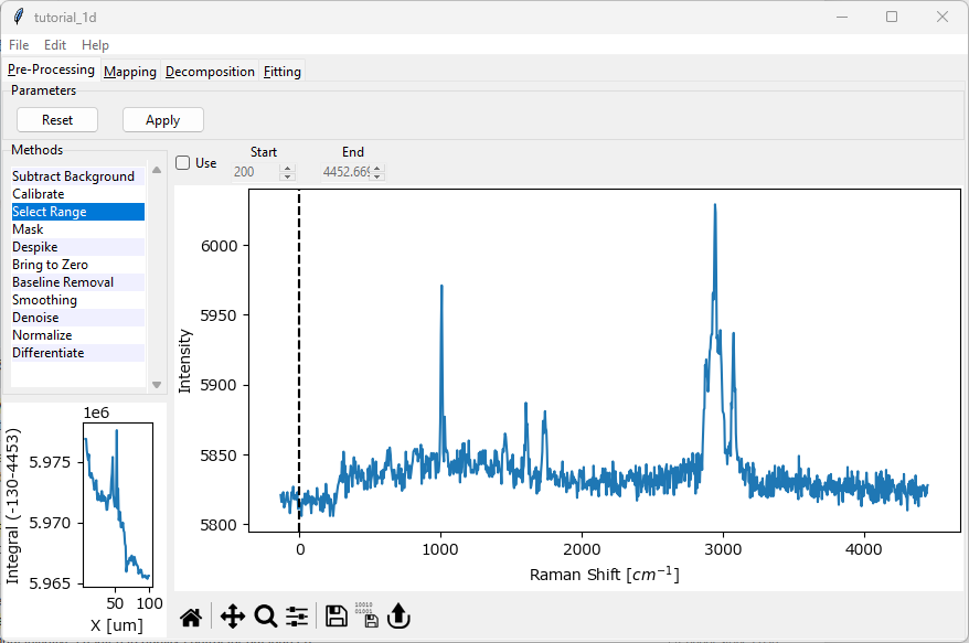
Fig. 2.1 The Tutorial Dataset

After loading the data, your screen should look similar to the figure above. This is the preprocessing screen.
Since we don’t know anything about our dataset (yet), we will keep initial preprocessing to a minimum:

1. chose Select Range from the Methods list on the left if it is not already selected.

2. click the Use checkbox to enable the Select Range preprocessing step.

3. select the region between approximately 360 cm^-1 and 3500 cm^-1. You can do this by typing these numbers into the Start and Stop boxes or by dragging the dashed line Controls in the graph.

4. Click the Apply button to perform the preprocessing steps.

Select Range simply selects the spectral range of interest. Here, we are removing the empty spectral region > 3500 cm^-1 and the low-wavenumber region masked by the bandpass filter < 300 cm^-1. You screen should now look like the this

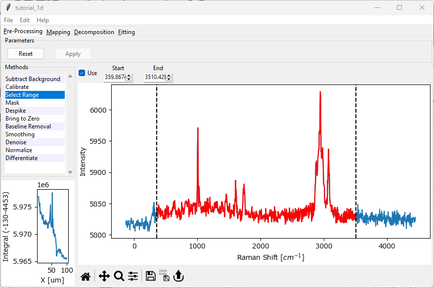
Fig. 2.2 The Tutorial Dataset - Range Selection

Next, we switch to the Mapping tab. The Mapping tab allows plotting various spectral parameters, for example band intensity or intensity ratios. You can switch to the Mapping tab by clicking Mapping in the top tab row of the SMDExplorer window.

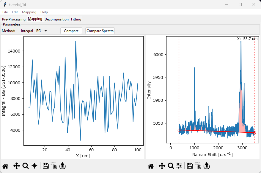
Fig. 2.3 The Tutorial Dataset - Data Exploration

The Mapping screen contains two panes:

• the left pane contains an intensity profile / mapping of the dataset. Right now, we are plotting the integrated intensity of the entire spectrum (minus a background) versus the spatial (x) coordinate of the line scan.

• the right pane contains the selected spectrum.

You can change the spectrum displayed in the right pane by clicking in the left pane. In this tutorial, we would like to compare a spectrum at the beginning of the line scan, for example at x=5 μm, with a spectrum at the end of the line scan, for example at x=95 μm. To do this

1. click and drag in the left (profile) pane and select a spectrum at the left, lower x end of the data. The red vertical bar indicates the selected spectrum and the coordinate of the displayed spectrum in the right pane will update along with the spectrum.

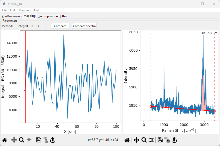
Fig. 2.4 Selecting a spectrum

2. Click the Compare Spectra button. A new window will open displaying the selected spectrum.

3. Do the same for a spectrum at the upper end of the x range and click Compare Spectra again.

4. The second spectrum will be appended to the comparison window.

The comparison window should now look like this

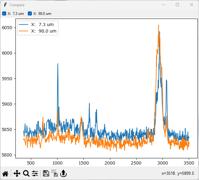
Fig. 2.5 Comparing Spectra

It is clear that there are spectral differences between spectra at low x and high x. To have a closer look:

1. click the Lupe icon at the bottom toolbar of the comparison window to turn on Zoom mode.

2. Zoom into the region between 2600 cm^-1 and 3300 cm^-1. To do this, click and drag in the graph to draw a rectangle that spans this region.

   

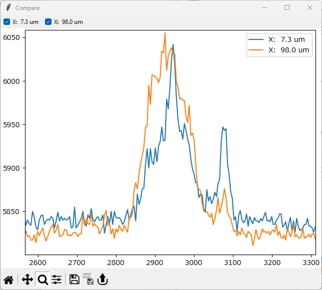
   Fig. 2.6 Comparing Spectra - Zooming

   There clearly are spectral differences in the CH₂-stretching region of the Raman spectra.

3. Turn off Zoom by clicking the Lupe icon again.

4. Return to the full-range view by clicking the Autoscale button (the little house at the very left of the toolbar.)

5. (optional) explore the graphing functionality of SMDExplorer by navigating around the graph by zooming and panning. The Graphing section has details on mouse gestures and keyboard shortcuts that make this easy.

6. You can close the comparison window now.

Our superficial inspection has revealed spectral differences in the CH₂-stretching region of the Raman spectra around 3000 cm^-1. We can visualize this in the intensity profile.

1. in the Mapping window, select Integral-BG from the Method dropdown menu (if not already selected).

2. In the right spectrum pane, drag the vertical red dotted lines to flank the peak at around 3000 cm^-1.

3. The profile in the left pane will update and display the integrated intensity in the selected region after subtracting a linear baseline between the endpoints. The integrated intensity is indicated by the red shaded region in the graph.

4. The intensity profile should display a sigmoidal curve indicating an intensity increase in the CH₂-stretching region as we transition across the interface between the two organic materials.

   

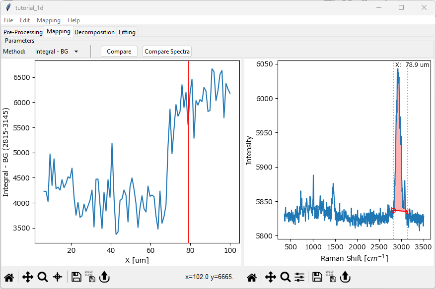
   Fig. 2.7 Plotting an Intensity Profile

5. (optional) explore some of the other image formation methods from the Method dropdown menu.

This concludes the first part of the SMDExplorer guided tour. In the next part, we will explore how to use SMDExplorer to plot intensity profiles in an automated, semi-unsupervised fashion.

2.2. Automated Image Formation

In the previous section, we have had a cursory look at the tutorial dataset. After slightly cropping the spectral range to remove instrumental artifacts, we visually identified spectral differences and plotted the integrated intensity to obtain an intensity profile.
In this section, we will try to automate most of this process using Automated Image Formation.

Video

This video contains the steps of the Automated Image Formation tutorial. Alternatively, follow the steps below.

1. To get started, navigate back got the preprocessing screen and click the Reset button to discard our previous preprocessing result.

   Note

   SMDExplorer will remember your settings.

2. Select Baseline Removal from the Methods sidebar and click Use to enable the Non-linear baseline subtraction preprocessing step.

   

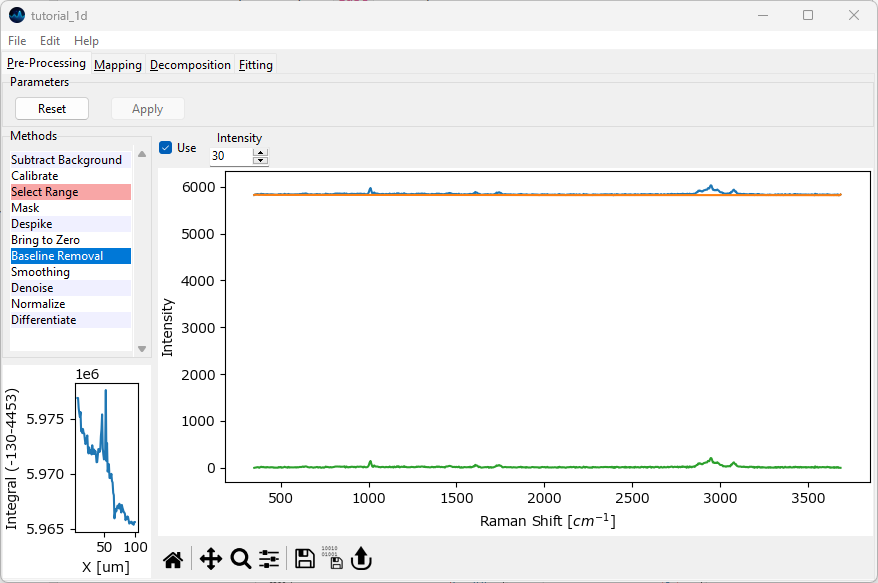
   Fig. 2.8 Non-linear baseline subtraction

   Feel free to zoom into the graph to get a close-up view of the calculated baseline. The default Intensity value is fine for this dataset.

3. Click Apply to process the data and navigate to the Decomposition screen by clicking on the Decomposition tab at the top of the window.

4. We will perform non-negative matrix decomposition to extract spectral components and their distribution from our dataset. In the Decomposition screen, select \(2\) for Number of Components, either by typing into the Number of Components field or by clicking the down arrow next to it. Leave the other parameters unchanged.

   See also

   The Automated Image Formation chapter provides a detailed explanation of the parameters.

5. Click the Apply button. The result should look like the figure below.

   

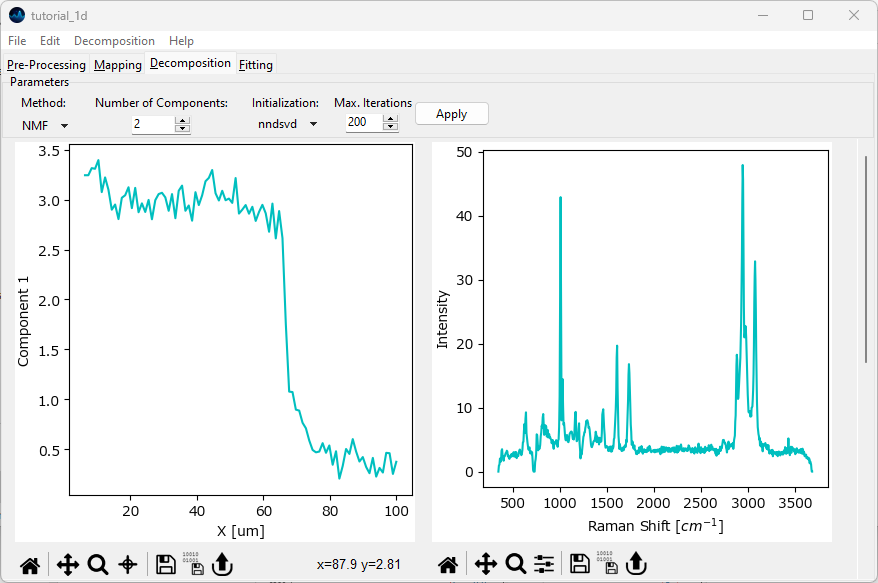
   Fig. 2.9 Automated Decomposition

   The algorithm has split the dataset into two components and extracted characteristic spectra as well as concentration profiles for each component. The first component has high intensity at low x values and starts decreasing around 70 μm. The second component starts increasing around 70 μm from a low to a high concentration. You might have to scroll down to see the second component.

6. This observation matches our findings when inspecting the data manually. To compare the two spectra, select Show Overlay from the Decomposition menu. In the Overlay window, activate the checkboxes for Component 1 and Component 2 to display all extracted components.

   

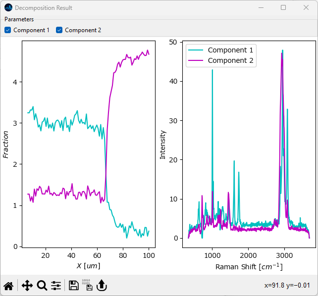
   Fig. 2.10 Comparing Decompostion Results

   You should see a graph like the one shown above. The left panel displays the concentrations (in arbitrary units) of the two components, the left panel contains their spectra. Feel free to zoom into the spectra graph on the left to check the spectral differences between the two components.

   Tip

   Notice the vastly improved signal-to-noise ratio of the extracted spectra compared to the raw data.

Note

Automated image formation is a great way to explore an unknown dataset. See the Automated Image Formation - A How-to section for more detailed instructions and caveats.

This concludes the second part of the SMDExplorer guided tour. In the next part, we will try to replicate the automated image formation result by ratiometric imaging and explore some further preprocessing options in the process.

2.3. Ratiometric Imaging

In the previous section, we have used automated image formation to perform an initial assessment of the tutorial dataset. In this chapter, we will build on this result to perform a more in depth manual analysis. At the same time, we will be exploring some additional data preprocessing options available in SMDExplorer.

Our initial assessment of the dataset has revealed that the spectra are quite noisy. SMDExplorer provides several options to improve the signal-to-noise ratio, which we will be exploring here.

Video

This video contains the steps of the Ratiometric Imaging tutorial. Alternatively, follow the steps below.

1. Return to the preprocessing screen and click Reset to discard the previous preprocessing result. Leave the Select Range and Baseline Removal steps active and deactivate all other preprocessing steps that might have been active.

2. Click Apply to perform cropping and baseline subtraction.

3. Navigate to the Mapping screen and select a spectrum by clicking and dragging in the left pane. Click Compare Spectra to add this spectrum to the comparison window.

   Note

   It does not matter which spectrum you select for this comparison.

4. Return to the preprocessing screen and click Reset to discard the previous preprocessing result. Select Smoothing from the Methods sidebar. Smoothing will remove noise from each spectrum by fitting a small spectral region with a low-degree polynomial. Activate the Smoothing preprocessing step by checking the Use checkbox. The orange trace in the preview window represents the smoothed spectrum.

   

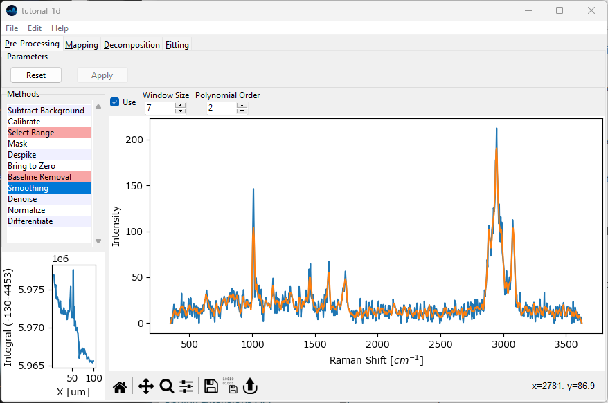
   Fig. 2.11 Spectral Smoothing

   Tip

   Explore the effect of Window Size and Polynomial Degree.

5. Click Apply to perform the three active preprocessing steps (Select Range, Baseline Removal, Smoothing) and return to the Mapping screen. Select the same spectrum as before by clicking and dragging in the left pane. Click Compare Spectra to add this spectrum to the comparison window.

   Tip

   The top right corner of the spectrum pane displays the x-coordinate of the spectrum. Observing this value should make it easy to select the same position.

   

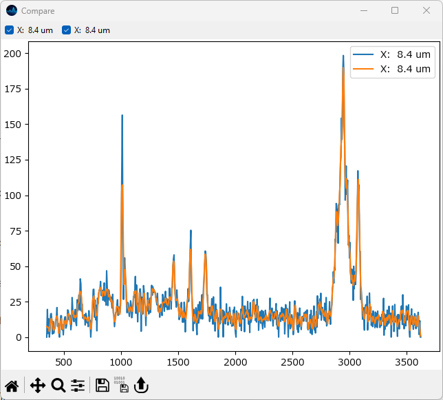
   Fig. 2.12 Comparing Smoothed Spectra

6. Navigate back to the Preprocessing window, click Reset to discard the previous result, deactivate Smoothing by unchecking Use in the smoothing pane, and select Denoise from the Methods sidebar. We will denoise the dataset by PCA denoising.

7. From the Mode menu, select Denoise. As Filter, select PCA. For Number of Components, select 4. Finally, activate the Denoise preprocessing step by checking Use and click Apply to perform the three active preprocessing steps.

   

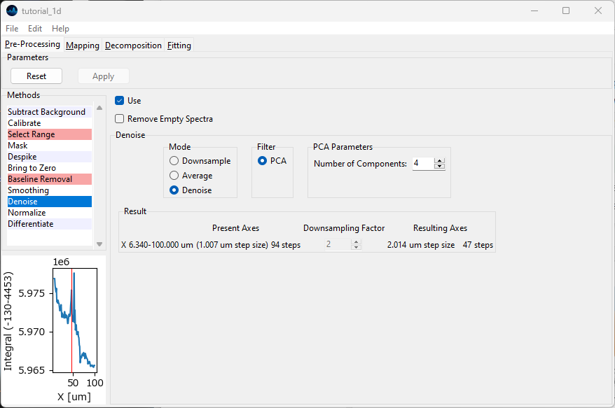
   Fig. 2.13 The Denoise Screen

   Hint

   Smoothing operates on individual spectra, Denoising on datasets of several spectra. The more spectra (with similar features) in the dataset, the better the denoising algorithm will perform. Since processing an entire dataset can potentially take a lot of time, there is no preview for Denoising.

8. Return to the Mapping screen, select the same spectrum as before, and add it to the comparison by clicking the Compare Spectra button.

9. Inspect the smoothed / denoised spectra.

   

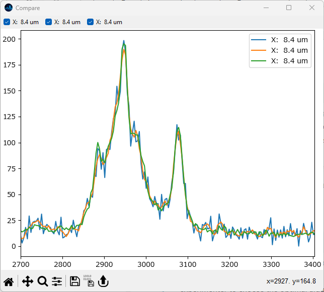
   Fig. 2.14 Comparing Smoothed / Denoised Spectra

   Note

   Selecting the appropriate smoothing / denoising procedure highly depends on the dataset, the amount of noise, and the number of spectra recorded. Ultimately, it is up to the experimenter to choose the optimal algorithm. Please note that Smoothing and Denoising can be combined and that SMDExplorer offers additional Denoising methods.

   For the tutorial dataset, PCA Denoising performs very well. We will continue to use the denoised dataset for the remainder of this section of the tutorial.

10. In the Mapping screen, select Ratio from the Method dropdown menu. This will make two additional, green Controls appear in the spectrum window. Drag all of the controls (dotted vertical lines) in the region around the peak at 3000 cm^-1 and then zoom in to make this peak easier to see.

11. Using the green control, select the region between approximately 2850 cm^-1 and 3030 cm^-1. With the red control, select the region from 3030 cm^-1 and 3115 cm^-1. Your screen should now resemble the figure below

    

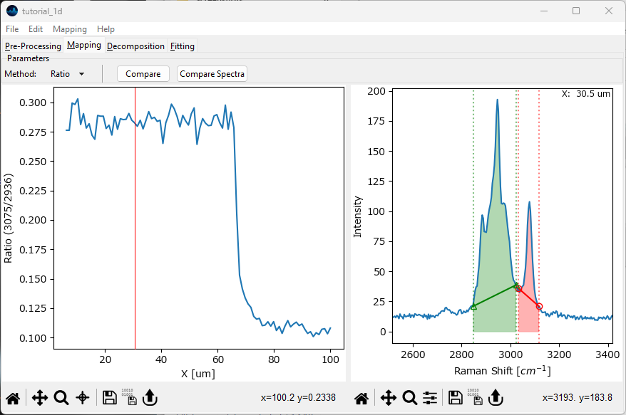
    Fig. 2.15 Plotting a peak ratio

    The left pane now contains the quotient of the red shaded area and the green shaded area.

    Important

    Ratio computes the quotient of two running sums that include the baseline of the spectrum. If the baseline is offset significantly from zero, or varies throughout the dataset, this is generally not what you want. Here, we have subtracted the baseline by non-linear baseline removal so computing the ratio this way is valid.
    (optional) turn of baseline subtraction an perform the same analysis.

12. Select Ratio - BG from the Method dropdown menu. Like Ratio, this computes the quotient between the integral of two areas but additionally subtracts the linear baseline between the endpoints of the selected region. The red and green shaded regions represent the enumerator and denominator of the quotient.

    

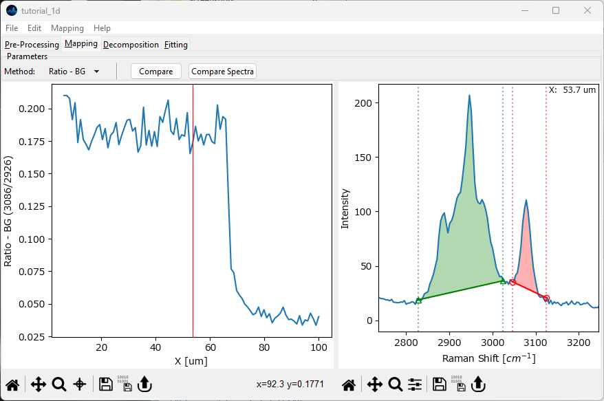
    Fig. 2.16 Plotting a peak ratio - background subtraction

    Note

    The additional baseline calculation step makes Ratio - BG more sensitive to noise.

This concludes the third part of the SMDExplorer tutorial. In the next part, we will explore peak deconvolution.

2.4. Peak Deconvolution

In this section, we will explore the peak deconvolution functionality of SMDExplorer. Peak deconvolution allows separating overlapping peaks by curve fitting.

See also

The section Peak Deconvolution - A How-to contains a detailed tutorial beyond this introduction.

Video

This video contains the steps of the Peak Deconvolution tutorial. Alternatively, follow the steps below.

1. Navigate to the Preprocessing screen and deactivate the Denoising and Baseline Removal steps. In the Range Selection screen, select the spectral region between approximately 2650 cm ^-1 and 3500 cm ^-1. Click Reset (if required) and Apply to crop the spectrum to the CH₂ stretching region.

   

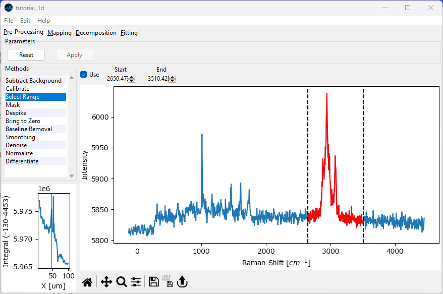
   Fig. 2.17 Selecting the spectral region for fitting

2. Navigate to the Peak Deconvolution screen by clicking Fitting in the top tab bar.

3. In the fitting screen, select the spectrum at x = 22.5 μm by clicking and dragging in the right-most pane.

   Note

   This tutorial will work with any other selected spectrum as well. Selecting the same spectrum, however, will make it easier to follow along.

4. We will have SMDExplorer guess peak the positions to speed up the curve fitting procedure. To do this, click the Update Autoguess button to initialize the autoguess algorithm with the current spectrum. Then, use the slider above the Update Autoguess button to adjust the sensitivity. Moving the slider to the left will increase sensitivity, moving the slider to the right will decrease sensitivity. Adjust the slider until the three most prominent peaks have been detected.

   

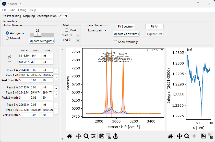
   Fig. 2.18 Peak Deconvolution - Initial Guesses

5. Select Lorentzian from the Line Shape dropdown menu. Click the Fit Spectrum button to fit the spectrum with the currently specified three peaks.

   

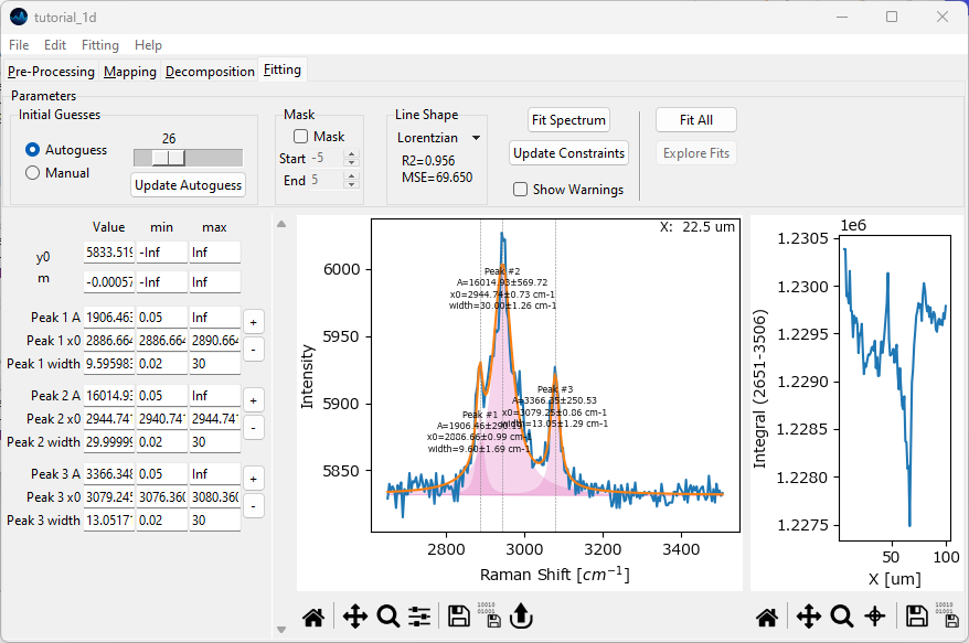
   Fig. 2.19 Peak Deconvolution - First Fit

   The initial fit is not bad, but we can do better. Zooming in reveals that we should add one or more peaks to better reproduce the data.

   Important

   Peaks in the tutorial dataset change significantly in terms of position and amplitude. For best results, fitting should be performed using constraints. Please make sure that the Use Constraints checkbox is activated before proceeding and that the default constraint level is set to tight constraints.

6. Click the + button next to Peak 2 in the leftmost Fit Coefficients pane and add a peak centered at 2995 cm^-1. Do this by entering 2995 into the window that pops up after clicking the + and selecting OK.

7. Add another peak at 2920 cm^-1 in the same fashion.

8. Both peaks have been added to the set of fit coefficients. Click Fit Spectrum button to update the fit. The resulting orange fit curve should reproduce the shape of the spectrum better now.

9. Click the Update Constraints button followed by the Fit Spectrum button. Do this until the fit curve appears stable.

   

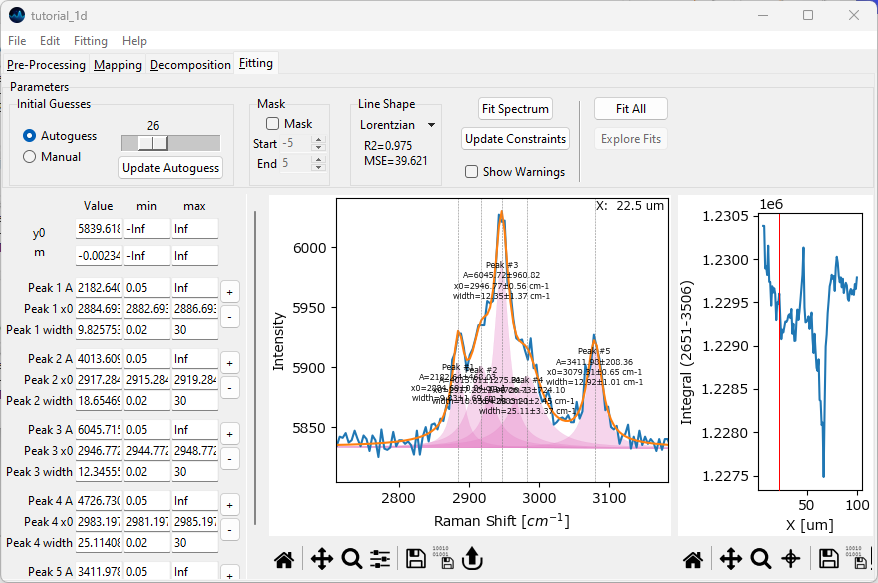
   Fig. 2.20 Peak Deconvolution - Adding Peaks

10. Select a different spectrum by clicking and dragging in the right-most pane. Click the Fit Spectrum button to check how the current set of initial guesses fits the data.

11. (optional) optimize fitting constraints. To do this, activate the Show Warnings checkbox. If a peak is being limited by the parameter constrains (minimum and maximum), a warning will be displayed. Adjust the upper or lower limit for this peak and parameter accordingly.

    See also

    The section Peak Deconvolution - A How-to contains more details how to handle constraints.

12. If you feel that the set of initial guesses in the Fit Coefficients pane provides good fitting results for the entire dataset, click the Fit All button to fit all spectra with the selected set of five peaks. Once all 100 spectra have been fit, you can click and drag in the right-most pane to see the result for each spectrum.

13. Click the Explore Fits button to open the Peak Deconvolution Analysis Window. Activate the Show Spectra checkbox to display spectra and their peak deconvolution result.

14. Visualize the intensity profile of the peak centered at 3080 cm ^-1 (the rightmost peak, peak number 5 in this example). To do this, select this peak from the Peak 1# dropdown. The correct peak number is displayed above the peak in the right-hand pane. Next, select Amplitude to plot the peak’s amplitude.

    

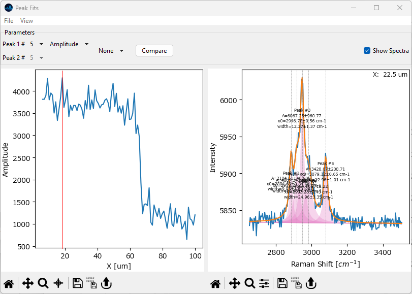
    Fig. 2.21 Peak Deconvolution - Visualization

15. Visualize the ratio between the peaks centered at 3080 cm ^-1 and 2945 cm ^-1. To do this, select Ratio from the Operation dropdown menu and select the correct peak from the Peak 2# dropdown. In this example, the peak centered at 2945 cm ^-1 is peak 3.

    

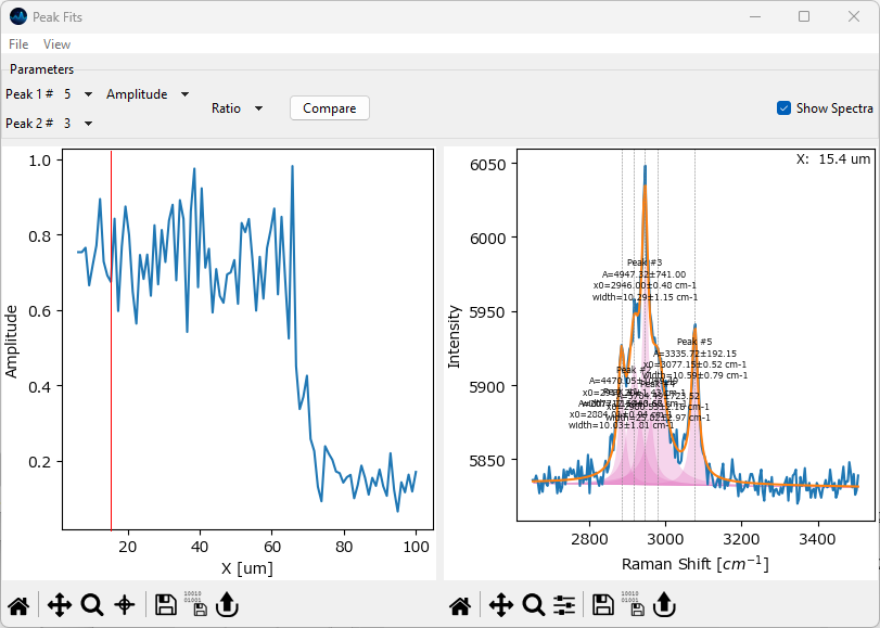
    Fig. 2.22 Peak Deconvolution - Visualization an Amplitude Ratio

16. (optional) Explore and visualize other parameters extracted form the dataset, such as peak positions and peak widths.

Important

This tutorial is designed to provide an introduction into peak deconvolution. For proper analysis of this dataset, especially peak positions, optimization of constraints is essential. SMDExplorer tries to make this as easy as possible, but if you find the default positional constraints too limiting, the allowable range can be adjusted in Preferences.

This concludes the guided tour of SMDExplorer. Please see the following chapters for further details on how to analyze spectral data.